SYSTEMS OF LINEAR EQUATIONS
I. Statement of the problem.
II. Compatibility of homogeneous and heterogeneous systems.
III. System T equations with T unknown. Cramer's rule.
IV. Matrix method for solving systems of equations.
V. Gauss method.
I. Statement of the problem.
A system of equations of the form
called a system m
linear equations With n unknown  . The coefficients of the equations of this system are written in the form of a matrix

which is called matrix of the system (1).
The numbers on the right sides of the equations form free members column {B}:
 .
.
If column ( B}={0 ), then the system of equations is called homogeneous. Otherwise, when ( B}≠{0 ) - system heterogeneous.
System of linear equations (1) can be written in matrix form
[A]{x}={B}. (2)
Here  - column of unknowns.
Solving the system of equations (1) means finding the set n
numbers  such that when substituting into system (1) instead of the unknowns
  Each equation of the system turns into an identity. Numbers
  are called the solution of a system of equations.
A system of linear equations can have one solution
 ,
,
can have countless solutions

or have no solutions at all
 .
.
Systems of equations that have no solutions are called incompatible. If a system of equations has at least one solution, then it is called joint. The system of equations is called certain, if it has a unique solution, and uncertain, if it has infinitely many solutions.
II. Compatibility of homogeneous and heterogeneous systems.
The compatibility condition for the system of linear equations (1) is formulated in Kronecker-Capelli theorem: a system of linear equations has at least one solution if and only if the rank of the system matrix is equal to the rank of the extended matrix:  .
.
An extended system matrix is a matrix obtained from the system matrix by adding a column of free terms to it on the right:
 .
.
If Rg A
Homogeneous systems of linear equations, in accordance with the Kronecker-Capelli theorem, are always consistent. Let us consider the case of a homogeneous system in which the number of equations is equal to the number of unknowns, that is t=p. If the determinant of the matrix of such a system is not equal to zero, i.e.  , a homogeneous system has a unique solution, which is trivial (zero). Homogeneous systems have an infinite number of solutions if among the equations of the system there are linearly dependent ones, i.e.
  .
.
Example. Consider a homogeneous system of three linear equations with three unknowns:

and examine the question of the number of its solutions. Each of the equations can be considered an equation of a plane passing through the origin of coordinates ( D=0 ). The system of equations has a unique solution when all three planes intersect at one point. Moreover, their normal vectors are non-coplanar, and, therefore, the condition is satisfied
 .
.
The solution of the system in this case x=0, y=0, z=0 .
If at least two of the three planes, for example, the first and second, are parallel, i.e. , then the determinant of the system matrix is equal to zero, and the system has an infinite number of solutions. Moreover, the solutions will be the coordinates x, y, z all points lying on a line

If all three planes coincide, then the system of equations will be reduced to one equation
 ,
,
and the solution will be the coordinates of all points lying in this plane.
When studying inhomogeneous systems of linear equations, the question of compatibility is solved using the Kronecker-Capelli theorem. If the number of equations in such a system is equal to the number of unknowns, then the system has a unique solution if its determinant is not equal to zero. Otherwise, the system is either inconsistent or has an infinite number of solutions.
Example. We study an inhomogeneous system of two equations with two unknowns
 .
.
The equations of the system can be considered as equations of two lines on a plane. The system is inconsistent when the lines are parallel, i.e.
 ,
,
 . In this case, the rank of the system matrix is 1:
Rg A=1
, because  ,
,
and the rank of the extended matrix  is equal to two, since for it a second-order minor containing the third column can be chosen as a basis minor.
In the case under consideration, Rg A
If the lines coincide, i.e. , then the system of equations has an infinite number of solutions: coordinates of points on a straight line  . In this case, Rg A=
Rg A *
=1.
. In this case, Rg A=
Rg A *
=1.
The system has a unique solution when the lines are not parallel, i.e.  . The solution to this system is the coordinates of the point of intersection of the lines
III. SystemT equations withT unknown. Cramer's rule.
Let us consider the simplest case when the number of equations of the system is equal to the number of unknowns, i.e. m= n. If the determinant of the system matrix is nonzero, the solution to the system can be found using Cramer's rule:
 (3)
(3)
Here  - determinant of the system matrix,
 is the determinant of the matrix obtained from [ A] replacement i th column to the column of free members:
 .
.
Example. Solve the system of equations using Cramer's method.

Solution :
1) find the determinant of the system

2) find auxiliary determinants

3) find a solution to the system using Cramer’s rule:

The result of the solution can be checked by substituting into the system of equations

The correct identities are obtained.
IV. Matrix method for solving systems of equations.
Let us write the system of linear equations in matrix form (2)
[A]{x}={B}
and multiply the right and left sides of relation (2) on the left by the matrix [ A -1 ], inverse of the system matrix:
[A -1 ][A]{x}=[A -1 ]{B}. (2)
By definition of the inverse matrix, the product [ A -1 ][A]=[E], and according to the properties of the identity matrix [ E]{x}={x). Then from relation (2") we obtain
{x}=[A -1 ]{B}. (4)
Relation (4) underlies the matrix method for solving systems of linear equations: it is necessary to find the matrix inverse to the matrix of the system and multiply the column vector of the right parts of the system by it on the left.
Example. Let us solve the system of equations considered in the previous example using the matrix method.

System Matrix  its determinant det A==183
.
its determinant det A==183
.
Right side column
 .
.
To find the matrix [ A -1 ], find the matrix attached to [ A]:

or 
The formula for calculating the inverse matrix includes  , Then

Now we can find a solution to the system

Then we finally get  .
.
V. Gauss method.
With a large number of unknowns, solving a system of equations using the Cramer method or the matrix method involves calculating high-order determinants or inverting large matrices. These procedures are very labor-intensive even for modern computers. Therefore, to solve systems of a large number of equations, the Gauss method is often used.
The Gaussian method consists of sequentially eliminating unknowns through elementary transformations of the extended matrix of the system. Elementary matrix transformations include permutation of rows, addition of rows, multiplication of rows by numbers other than zero. As a result of the transformations, it is possible to reduce the matrix of the system to an upper triangular one, on the main diagonal of which there are ones, and below the main diagonal there are zeros. This is the direct approach of the Gaussian method. The reverse of the method consists in directly determining the unknowns, starting from the last one.
Let us illustrate the Gauss method using the example of solving a system of equations

At the first step of the forward stroke, it is ensured that the coefficient  transformed system became equal 1
, and the coefficients
transformed system became equal 1
, and the coefficients  And
And  turned to zero. To do this, multiply the first equation by 1/10
, multiply the second equation by 10
and add it to the first one, multiply the third equation by -10/2
and add it to the first one. After these transformations we get
turned to zero. To do this, multiply the first equation by 1/10
, multiply the second equation by 10
and add it to the first one, multiply the third equation by -10/2
and add it to the first one. After these transformations we get

At the second step, we ensure that after transformations the coefficient  became equal 1
, and the coefficient
became equal 1
, and the coefficient  . To do this, divide the second equation by 42
, and multiply the third equation by -42/27
and add it with the second one. We obtain a system of equations
. To do this, divide the second equation by 42
, and multiply the third equation by -42/27
and add it with the second one. We obtain a system of equations

At the third step we should get the coefficient  . To do this, divide the third equation by (37 - 84/27)
; we get
. To do this, divide the third equation by (37 - 84/27)
; we get

This is where the direct progression of the Gauss method ends, because the matrix of the system is reduced to the upper triangular one:

Carrying out the reverse move, we find the unknowns

Linear equations in two variables
A schoolchild has 200 rubles to eat lunch at school. A cake costs 25 rubles, and a cup of coffee costs 10 rubles. How many cakes and cups of coffee can you buy for 200 rubles?
Let us denote the number of cakes by x, and the number of cups of coffee through y. Then the cost of the cakes will be denoted by the expression 25 x, and the cost of cups of coffee in 10 y .
25x— price x cakes
10y — price y cups of coffee
The total amount should be 200 rubles. Then we get an equation with two variables x And y
25x+ 10y= 200
How many roots does this equation have?
It all depends on the student’s appetite. If he buys 6 cakes and 5 cups of coffee, then the roots of the equation will be the numbers 6 and 5.
The pair of values 6 and 5 are said to be the roots of equation 25 x+ 10y= 200 . Written as (6; 5), with the first number being the value of the variable x, and the second - the value of the variable y .
6 and 5 are not the only roots that reverse equation 25 x+ 10y= 200 to identity. If desired, for the same 200 rubles a student can buy 4 cakes and 10 cups of coffee:

In this case, the roots of equation 25 x+ 10y= 200 is a pair of values (4; 10).
Moreover, a schoolchild may not buy coffee at all, but buy cakes for the entire 200 rubles. Then the roots of equation 25 x+ 10y= 200 will be the values 8 and 0

Or vice versa, don’t buy cakes, but buy coffee for the entire 200 rubles. Then the roots of equation 25 x+ 10y= 200 the values will be 0 and 20

Let's try to list all possible roots of equation 25 x+ 10y= 200 . Let us agree that the values x And y belong to the set of integers. And let these values be greater than or equal to zero:
x∈Z, y∈ Z;
x ≥ 0, y ≥ 0
This will be convenient for the student himself. It is more convenient to buy whole cakes than, for example, several whole cakes and half a cake. It is also more convenient to take coffee in whole cups than, for example, several whole cups and half a cup.
Note that for odd x it is impossible to achieve equality under any circumstances y. Then the values x the following numbers will be 0, 2, 4, 6, 8. And knowing x can be easily determined y

Thus, we received the following pairs of values (0; 20), (2; 15), (4; 10), (6; 5), (8; 0). These pairs are solutions or roots of Equation 25 x+ 10y= 200. They turn this equation into an identity.
Equation of the form ax + by = c called linear equation with two variables. The solution or roots of this equation are a pair of values ( x; y), which turns it into identity.
Note also that if a linear equation with two variables is written in the form ax + b y = c , then they say that it is written in canonical(normal) form.
Some linear equations in two variables can be reduced to canonical form.
For example, the equation 2(16x+ 3y − 4) = 2(12 + 8x − y) can be brought to mind ax + by = c. Let's open the brackets on both sides of this equation and get 32x + 6y − 8 = 24 + 16x − 2y . We group terms containing unknowns on the left side of the equation, and terms free of unknowns - on the right. Then we get 32x− 16x+ 6y+ 2y = 24 + 8 . We present similar terms in both sides, we get equation 16 x+ 8y= 32. This equation is reduced to the form ax + by = c and is canonical.
Equation 25 discussed earlier x+ 10y= 200 is also a linear equation with two variables in canonical form. In this equation the parameters a , b And c are equal to the values 25, 10 and 200, respectively.
Actually the equation ax + by = c has countless solutions. Solving the equation 25x+ 10y= 200, we looked for its roots only on the set of integers. As a result, we obtained several pairs of values that turned this equation into an identity. But on the set of rational numbers, equation 25 x+ 10y= 200 will have infinitely many solutions.
To obtain new pairs of values, you need to take an arbitrary value for x, then express y. For example, let's take for the variable x value 7. Then we get an equation with one variable 25×7 + 10y= 200 in which one can express y

Let x= 15. Then the equation 25x+ 10y= 200 becomes 25 × 15 + 10y= 200. From here we find that y = −17,5

Let x= −3 . Then the equation 25x+ 10y= 200 becomes 25 × (−3) + 10y= 200. From here we find that y = −27,5

System of two linear equations with two variables
For the equation ax + by = c you can take arbitrary values for as many times as you like x and find values for y. Taken separately, such an equation will have countless solutions.
But it also happens that the variables x And y connected not by one, but by two equations. In this case they form the so-called system of linear equations in two variables. Such a system of equations can have one pair of values (or in other words: “one solution”).
It may also happen that the system has no solutions at all. A system of linear equations can have countless solutions in rare and exceptional cases.
Two linear equations form a system when the values x And y enter into each of these equations.
Let's go back to the very first equation 25 x+ 10y= 200 . One of the pairs of values for this equation was the pair (6; 5) . This is a case when for 200 rubles you could buy 6 cakes and 5 cups of coffee.
Let's formulate the problem so that the pair (6; 5) becomes the only solution for equation 25 x+ 10y= 200 . To do this, let’s create another equation that would connect the same x cakes and y cups of coffee.
Let us state the text of the problem as follows:
“The student bought several cakes and several cups of coffee for 200 rubles. A cake costs 25 rubles, and a cup of coffee costs 10 rubles. How many cakes and cups of coffee did the student buy if it is known that the number of cakes is one unit greater than the number of cups of coffee?
We already have the first equation. This is equation 25 x+ 10y= 200 . Now let's create an equation for the condition “the number of cakes is one unit greater than the number of cups of coffee” .
The number of cakes is x, and the number of cups of coffee is y. You can write this phrase using the equation x−y= 1. This equation will mean that the difference between cakes and coffee is 1.
x = y+ 1 . This equation means that the number of cakes is one more than the number of cups of coffee. Therefore, to obtain equality, one is added to the number of cups of coffee. This can be easily understood if we use the model of scales that we considered when studying the simplest problems:

We got two equations: 25 x+ 10y= 200 and x = y+ 1. Since the values x And y, namely 6 and 5 are included in each of these equations, then together they form a system. Let's write down this system. If the equations form a system, then they are framed by the system sign. The system symbol is a curly brace:

Let's solve this system. This will allow us to see how we arrive at the values 6 and 5. There are many methods for solving such systems. Let's look at the most popular of them.
Substitution method
The name of this method speaks for itself. Its essence is to substitute one equation into another, having previously expressed one of the variables.
In our system, nothing needs to be expressed. In the second equation x = y+ 1 variable x already expressed. This variable is equal to the expression y+ 1 . Then you can substitute this expression into the first equation instead of the variable x

After substituting the expression y+ 1 into the first equation instead x, we get the equation 25(y+ 1) + 10y= 200 . This is a linear equation with one variable. This equation is quite easy to solve:

We found the value of the variable y. Now let's substitute this value into one of the equations and find the value x. For this it is convenient to use the second equation x = y+ 1 . Let’s substitute the value into it y
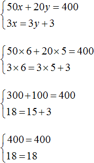
This means that the pair (6; 5) is a solution to the system of equations, as we intended. We check and make sure that the pair (6; 5) satisfies the system:

Example 2

Let's substitute the first equation x= 2 + y into the second equation 3 x− 2y= 9. In the first equation the variable x equal to the expression 2 + y. Let’s substitute this expression into the second equation instead of x

Now let's find the value x. To do this, let's substitute the value y into the first equation x= 2 + y
This means that the solution to the system is the pair value (5; 3)
Example 3. Solve the following system of equations using the substitution method:

Here, unlike previous examples, one of the variables is not expressed explicitly.
To substitute one equation into another, you first need .
It is advisable to express the variable that has a coefficient of one. The variable has a coefficient of one x, which is contained in the first equation x+ 2y= 11. Let's express this variable.
After variable expression x, our system will take the following form:

Now let's substitute the first equation into the second and find the value y

Let's substitute y x

This means that the solution to the system is a pair of values (3; 4)
Of course, you can also express a variable y. This will not change the roots. But if you express y, The result is not a very simple equation, which will take more time to solve. It will look like this:

We see that in this example we express x much more convenient than expressing y .
Example 4. Solve the following system of equations using the substitution method:

Let us express in the first equation x. Then the system will take the form:

y

Let's substitute y into the first equation and find x. You can use the original equation 7 x+ 9y= 8, or use the equation in which the variable is expressed x. We will use this equation because it is convenient:
![]()
This means that the solution to the system is a pair of values (5; −3)
Addition method
The addition method consists of adding the equations included in the system term by term. This addition results in a new equation with one variable. And solving such an equation is quite simple.
Let's solve the following system of equations:

Let's add the left side of the first equation with the left side of the second equation. And the right side of the first equation with the right side of the second equation. We get the following equality:
Let's look at similar terms:

As a result, we got the simplest equation 3 x= 27 whose root is 9. Knowing the value x you can find the value y. Let's substitute the value x into the second equation x−y= 3 . We get 9 − y= 3 . From here y= 6 .
This means that the solution to the system is a pair of values (9; 6)
Example 2

Let's add the left side of the first equation with the left side of the second equation. And the right side of the first equation with the right side of the second equation. In the resulting equality we present similar terms:

As a result, we got the simplest equation 5 x= 20, whose root is 4. Knowing the value x you can find the value y. Let's substitute the value x into the first equation 2 x+y= 11. Let's get 8+ y= 11. From here y= 3 .
This means that the solution to the system is a pair of values (4;3)
The addition process is not described in detail. It must be done mentally. When adding, both equations must be reduced to canonical form. That is, by the way ac + by = c .
From the examples considered, it is clear that the main purpose of adding equations is to get rid of one of the variables. But it is not always possible to immediately solve a system of equations using the addition method. Most often, the system is first brought to a form in which the equations included in this system can be added.
For example, the system  can be solved immediately by addition. When adding both equations, the terms y And −y will disappear because their sum is zero. As a result, the simplest equation 11 is formed x= 22, whose root is 2. It will then be possible to determine y equal to 5.
And the system of equations  The addition method cannot be solved immediately, since this will not lead to the disappearance of one of the variables. Addition will result in equation 8 x+ y= 28, which has an infinite number of solutions.
If both sides of the equation are multiplied or divided by the same number, not equal to zero, you get an equation equivalent to the given one. This rule is also true for a system of linear equations with two variables. One of the equations (or both equations) can be multiplied by any number. The result will be an equivalent system, the roots of which will coincide with the previous one.
Let's return to the very first system, which described how many cakes and cups of coffee a schoolchild bought. The solution to this system was a pair of values (6; 5).
Let's multiply both equations included in this system by some numbers. Let's say we multiply the first equation by 2, and the second by 3

As a result, we got a system 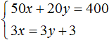
The solution to this system is still the pair of values (6; 5)
This means that the equations included in the system can be reduced to a form suitable for applying the addition method.
Let's return to the system , which we could not solve using the addition method.
Multiply the first equation by 6, and the second by −2

Then we get the following system:

Let's add up the equations included in this system. Adding components 12 x and −12 x will result in 0, addition 18 y and 4 y will give 22 y, and adding 108 and −20 gives 88. Then we get equation 22 y= 88, from here y = 4 .
If at first it’s hard to add equations in your head, then you can write down how the left side of the first equation adds up with the left side of the second equation, and the right side of the first equation with the right side of the second equation:

Knowing that the value of the variable y equals 4, you can find the value x. Let's substitute y into one of the equations, for example into the first equation 2 x+ 3y= 18. Then we get an equation with one variable 2 x+ 12 = 18. Let's move 12 to the right side, changing the sign, we get 2 x= 6, from here x = 3 .
Example 4. Solve the following system of equations using the addition method:

Let's multiply the second equation by −1. Then the system will take the following form:

Let's add both equations. Adding components x And −x will result in 0, addition 5 y and 3 y will give 8 y, and adding 7 and 1 gives 8. The result is equation 8 y= 8 whose root is 1. Knowing that the value y equals 1, you can find the value x .
Let's substitute y into the first equation, we get x+ 5 = 7, hence x= 2
Example 5. Solve the following system of equations using the addition method:

It is desirable that terms containing the same variables be located one below the other. Therefore, in the second equation the terms 5 y and −2 x Let's swap places. As a result, the system will take the form:

Let's multiply the second equation by 3. Then the system will take the form:

Now let's add both equations. As a result of addition we obtain equation 8 y= 16, whose root is 2.
Let's substitute y into the first equation, we get 6 x− 14 = 40. Let's move the term −14 to the right side, changing the sign, and get 6 x= 54 . From here x= 9.
Example 6. Solve the following system of equations using the addition method:

Let's get rid of fractions. Multiply the first equation by 36, and the second by 12
In the resulting system  the first equation can be multiplied by −5, and the second by 8

Let's add up the equations in the resulting system. Then we get the simplest equation −13 y= −156 . From here y= 12. Let's substitute y into the first equation and find x

Example 7. Solve the following system of equations using the addition method:

Let us bring both equations to normal form. Here it is convenient to apply the rule of proportion in both equations. If in the first equation the right side is represented as , and the right side of the second equation as , then the system will take the form:

We have a proportion. Let's multiply its extreme and middle terms. Then the system will take the form:

Let's multiply the first equation by −3, and open the brackets in the second:

Now let's add both equations. As a result of adding these equations, we get an equality with zero on both sides:

It turns out that the system has countless solutions.
But we can’t just take arbitrary values from the sky for x And y. We can specify one of the values, and the other will be determined depending on the value we specify. For example, let x= 2 . Let's substitute this value into the system:

As a result of solving one of the equations, the value for y, which will satisfy both equations:

The resulting pair of values (2; −2) will satisfy the system:
Let's find another pair of values. Let x= 4. Let's substitute this value into the system:

You can tell by eye that the value y equals zero. Then we get a pair of values (4; 0) that satisfies our system:

Example 8. Solve the following system of equations using the addition method:

Multiply the first equation by 6 and the second by 12

Let's rewrite what's left:


Let's multiply the first equation by −1. Then the system will take the form:

Now let's add both equations. As a result of addition, equation 6 is formed b= 48, whose root is 8. Substitute b into the first equation and find a

System of linear equations with three variables
A linear equation with three variables includes three variables with coefficients, as well as an intercept term. In canonical form it can be written as follows:
ax + by + cz = d
This equation has countless solutions. By giving two variables different values, a third value can be found. The solution in this case is a triple of values ( x; y; z) which turns the equation into an identity.
If the variables x, y, z are interconnected by three equations, then a system of three linear equations with three variables is formed. To solve such a system, you can use the same methods that apply to linear equations with two variables: the substitution method and the addition method.
Example 1. Solve the following system of equations using the substitution method:

Let us express in the third equation x. Then the system will take the form:

Now let's do the substitution. Variable x is equal to the expression 3 − 2y − 2z . Let's substitute this expression into the first and second equations:

Let's open the brackets in both equations and present similar terms:

We have arrived at a system of linear equations with two variables. In this case, it is convenient to use the addition method. As a result, the variable y will disappear and we can find the value of the variable z
![]()
Now let's find the value y. To do this, it is convenient to use the equation − y+ z= 4. Substitute the value into it z

Now let's find the value x. To do this, it is convenient to use the equation x= 3 − 2y − 2z . Let's substitute the values into it y And z

Thus, the triple of values (3; −2; 2) is a solution to our system. By checking we make sure that these values satisfy the system:

Example 2. Solve the system using the addition method

Let's add the first equation with the second, multiplied by −2.
If the second equation is multiplied by −2, it takes the form −6x+ 6y − 4z = −4 . Now let's add it to the first equation:

We see that as a result of elementary transformations, the value of the variable was determined x. It is equal to one.
Let's return to the main system. Let's add the second equation with the third, multiplied by −1. If the third equation is multiplied by −1, it takes the form −4x + 5y − 2z = −1 . Now let's add it to the second equation:

We got the equation x− 2y= −1 . Let's substitute the value into it x which we found earlier. Then we can determine the value y

Now we know the meanings x And y. This allows you to determine the value z. Let's use one of the equations included in the system:

Thus, the triple of values (1; 1; 1) is the solution to our system. By checking we make sure that these values satisfy the system:

Problems on composing systems of linear equations
The task of composing systems of equations is solved by entering several variables. Next, equations are compiled based on the conditions of the problem. From the compiled equations they form a system and solve it. Having solved the system, it is necessary to check whether its solution satisfies the conditions of the problem.
Problem 1. A Volga car drove out of the city to the collective farm. She returned back along another road, which was 5 km shorter than the first. In total, the car traveled 35 km round trip. How many kilometers is the length of each road?
Solution
Let x— length of the first road, y- length of the second. If the car traveled 35 km round trip, then the first equation can be written as x+ y= 35. This equation describes the sum of the lengths of both roads.
It is said that the car returned along a road that was 5 km shorter than the first one. Then the second equation can be written as x− y= 5. This equation shows that the difference between the road lengths is 5 km.
Or the second equation can be written as x= y+ 5. We will use this equation.
Because the variables x And y in both equations denote the same number, then we can form a system from them:
Let's solve this system using some of the previously studied methods. In this case, it is convenient to use the substitution method, since in the second equation the variable x already expressed.
Substitute the second equation into the first and find y
Let's substitute the found value y in the second equation x= y+ 5 and we'll find x
The length of the first road was designated through the variable x. Now we have found its meaning. Variable x is equal to 20. This means that the length of the first road is 20 km.
And the length of the second road was indicated by y. The value of this variable is 15. This means the length of the second road is 15 km.
Let's check. First, let's make sure that the system is solved correctly:

Now let’s check whether the solution (20; 15) satisfies the conditions of the problem.
It was said that the car traveled a total of 35 km round trip. We add the lengths of both roads and make sure that the solution (20; 15) satisfies this condition: 20 km + 15 km = 35 km
The following condition: the car returned back along another road, which was 5 km shorter than the first . We see that solution (20; 15) also satisfies this condition, since 15 km is shorter than 20 km by 5 km: 20 km − 15 km = 5 km
When composing a system, it is important that the variables represent the same numbers in all equations included in this system.
So our system contains two equations. These equations in turn contain variables x And y, which represent the same numbers in both equations, namely road lengths of 20 km and 15 km.
Problem 2. Oak and pine sleepers were loaded onto the platform, 300 sleepers in total. It is known that all oak sleepers weighed 1 ton less than all pine sleepers. Determine how many oak and pine sleepers there were separately, if each oak sleeper weighed 46 kg, and each pine sleeper 28 kg.
Solution
Let x oak and y pine sleepers were loaded onto the platform. If there were 300 sleepers in total, then the first equation can be written as x+y = 300 .
All oak sleepers weighed 46 x kg, and the pine ones weighed 28 y kg. Since oak sleepers weighed 1 ton less than pine sleepers, the second equation can be written as 28y − 46x= 1000 . This equation shows that the difference in mass between oak and pine sleepers is 1000 kg.
Tons were converted to kilograms since the mass of oak and pine sleepers was measured in kilograms.
As a result, we obtain two equations that form the system

Let's solve this system. Let us express in the first equation x. Then the system will take the form:

Substitute the first equation into the second and find y

Let's substitute y into the equation x= 300 − y and find out what it is x

This means that 100 oak and 200 pine sleepers were loaded onto the platform.
Let's check whether the solution (100; 200) satisfies the conditions of the problem. First, let's make sure that the system is solved correctly:

It was said that there were 300 sleepers in total. We add up the number of oak and pine sleepers and make sure that the solution (100; 200) satisfies this condition: 100 + 200 = 300.
The following condition: all oak sleepers weighed 1 ton less than all pine sleepers . We see that the solution (100; 200) also satisfies this condition, since 46 × 100 kg of oak sleepers is lighter than 28 × 200 kg of pine sleepers: 5600 kg − 4600 kg = 1000 kg.
Problem 3. We took three pieces of copper-nickel alloy in ratios of 2: 1, 3: 1 and 5: 1 by weight. A piece weighing 12 kg was fused from them with a ratio of copper and nickel content of 4: 1. Find the mass of each original piece if the mass of the first is twice the mass of the second.
Where x* - one of the solutions to the inhomogeneous system (2) (for example (4)), (E−A+A) forms the kernel (null space) of the matrix A.
Let's do a skeletal decomposition of the matrix (E−A+A):
E−A + A=Q·S
Where Q n×n−r- rank matrix (Q)=n−r, S n−r×n-rank matrix (S)=n−r.
Then (13) can be written in the following form:
x=x*+Q·k, ∀ k ∈ Rn-r.
Where k=Sz.
So, procedure for finding a general solution systems of linear equations using a pseudoinverse matrix can be represented in the following form:
- Calculating the pseudoinverse matrix A + .
- We calculate a particular solution to the inhomogeneous system of linear equations (2): x*=A + b.
- We check the compatibility of the system. To do this, we calculate A.A. + b. If A.A. + b≠b, then the system is inconsistent. Otherwise, we continue the procedure.
- Let's figure it out E−A+A.
- Doing skeletal decomposition E−A + A=Q·S.
- Building a solution
x=x*+Q·k, ∀ k ∈ Rn-r.
Solving a system of linear equations online
The online calculator allows you to find the general solution to a system of linear equations with detailed explanations.
However, in practice two more cases are widespread:
– The system is inconsistent (has no solutions);
– The system is consistent and has infinitely many solutions.
Note : The term “consistency” implies that the system has at least some solution. In a number of problems, it is necessary to first examine the system for compatibility; how to do this, see the article on rank of matrices.
For these systems, the most universal of all solution methods is used - Gaussian method. In fact, the “school” method will also lead to the answer, but in higher mathematics it is customary to use the Gaussian method of sequential elimination of unknowns. Those who are not familiar with the Gaussian method algorithm, please study the lesson first Gaussian method for dummies.
The elementary matrix transformations themselves are exactly the same, the difference will be in the ending of the solution. First, let's look at a couple of examples when the system has no solutions (inconsistent).
Example 1
What immediately catches your eye about this system? The number of equations is less than the number of variables. If the number of equations is less than the number of variables, then we can immediately say that the system is either inconsistent or has infinitely many solutions. And all that remains is to find out.
The beginning of the solution is completely ordinary - we write down the extended matrix of the system and, using elementary transformations, bring it to a stepwise form:
![]()
(1) On the top left step we need to get +1 or –1. There are no such numbers in the first column, so rearranging the rows will not give anything. The unit will have to organize itself, and this can be done in several ways. I did this: To the first line we add the third line, multiplied by -1.
(2) Now we get two zeros in the first column. To the second line we add the first line multiplied by 3. To the third line we add the first line multiplied by 5.
(3) After the transformation has been completed, it is always advisable to see if it is possible to simplify the resulting strings? Can. We divide the second line by 2, at the same time getting the required –1 on the second step. Divide the third line by –3.
(4) Add the second line to the third line.
Probably everyone noticed the bad line that resulted from elementary transformations: ![]() . It is clear that this cannot be so. Indeed, let us rewrite the resulting matrix
. It is clear that this cannot be so. Indeed, let us rewrite the resulting matrix ![]() back to the system of linear equations:
back to the system of linear equations: ![]()
If, as a result of elementary transformations, a string of the form is obtained, where is a number other than zero, then the system is inconsistent (has no solutions).
How to write down the ending of a task? Let’s draw with white chalk: “as a result of elementary transformations, a string of the form , where ” is obtained and give the answer: the system has no solutions (inconsistent).
If, according to the condition, it is required to RESEARCH the system for compatibility, then it is necessary to formalize the solution in a more solid style using the concept matrix rank and the Kronecker-Capelli theorem.
Please note that there is no reversal of the Gaussian algorithm here - there are no solutions and there is simply nothing to find.
Example 2
Solve a system of linear equations ![]()
This is an example for you to solve on your own. Full solution and answer at the end of the lesson. I remind you again that your solution may differ from my solution; the Gaussian algorithm does not have strong “rigidity”.
Another technical feature of the solution: elementary transformations can be stopped At once, as soon as a line like , where . Let's consider a conditional example: suppose that after the first transformation the matrix is obtained ![]() . The matrix has not yet been reduced to echelon form, but there is no need for further elementary transformations, since a line of the form has appeared, where . The answer should be given immediately that the system is incompatible.
. The matrix has not yet been reduced to echelon form, but there is no need for further elementary transformations, since a line of the form has appeared, where . The answer should be given immediately that the system is incompatible.
When a system of linear equations has no solutions, this is almost a gift, due to the fact that a short solution is obtained, sometimes literally in 2-3 steps.
But everything in this world is balanced, and a problem in which the system has infinitely many solutions is just longer.
Example 3
Solve a system of linear equations ![]()
There are 4 equations and 4 unknowns, so the system can either have a single solution, or have no solutions, or have infinitely many solutions. Be that as it may, the Gaussian method will in any case lead us to the answer. This is its versatility.
The beginning is again standard. Let us write down the extended matrix of the system and, using elementary transformations, bring it to a stepwise form: ![]()
That's all, and you were afraid.
(1) Please note that all numbers in the first column are divisible by 2, so 2 is fine on the top left step. To the second line we add the first line, multiplied by –4. To the third line we add the first line, multiplied by –2. To the fourth line we add the first line, multiplied by –1.
Attention! Many may be tempted by the fourth line subtract first line. This can be done, but it is not necessary; experience shows that the probability of an error in calculations increases several times. Just add: To the fourth line add the first line multiplied by –1 – exactly!
(2) The last three lines are proportional, two of them can be deleted.
Here again we need to show increased attention, but are the lines really proportional? To be on the safe side (especially for a teapot), it would be a good idea to multiply the second line by –1, and divide the fourth line by 2, resulting in three identical lines. And only after that remove two of them.
As a result of elementary transformations, the extended matrix of the system is reduced to a stepwise form: ![]()
When writing a task in a notebook, it is advisable to make the same notes in pencil for clarity.
Let us rewrite the corresponding system of equations: ![]()
There is no smell of a “ordinary” single solution to the system here. There is no bad line either. This means that this is the third remaining case - the system has infinitely many solutions. Sometimes, according to the condition, it is necessary to investigate the compatibility of the system (i.e. prove that a solution exists at all), you can read about this in the last paragraph of the article How to find the rank of a matrix? But for now let’s go over the basics:
An infinite set of solutions to a system is briefly written in the form of the so-called general solution of the system .
We find the general solution of the system using the inverse of the Gaussian method.
First we need to define what variables we have basic, and what variables free. You don’t have to bother yourself with the terms of linear algebra, just remember that there are such basic variables And free variables.
Basic variables always “sit” strictly on the steps of the matrix.
In this example, the basic variables are and
Free variables are everything remaining variables that did not receive a step. In our case there are two of them: – free variables.
Now you need All basic variables express only through free variables.
The reverse of the Gaussian algorithm traditionally works from the bottom up.
From the second equation of the system we express the basic variable:
Now look at the first equation: ![]() . First we substitute the found expression into it:
. First we substitute the found expression into it: ![]()
It remains to express the basic variable in terms of free variables: ![]()
In the end we got what we needed - All basic variables ( and ) are expressed only through free variables: ![]()
Actually, the general solution is ready: ![]()
How to write the general solution correctly?
Free variables are written into the general solution “by themselves” and strictly in their places. In this case, free variables should be written in the second and fourth positions: ![]() .
.
The resulting expressions for the basic variables ![]() and obviously needs to be written in the first and third positions:
and obviously needs to be written in the first and third positions: ![]()
Giving free variables arbitrary values, you can find infinitely many private solutions. The most popular values are zeros, since the particular solution is the easiest to obtain. Let's substitute into the general solution: ![]()
– private solution.
Another sweet pair are ones, let’s substitute them into the general solution: ![]()
– another private solution.
It is easy to see that the system of equations has infinitely many solutions(since we can give free variables any values)
Each the particular solution must satisfy to each equation of the system. This is the basis for a “quick” check of the correctness of the solution. Take, for example, a particular solution and substitute it into the left side of each equation of the original system: ![]()
Everything must come together. And with any particular solution you receive, everything should also agree.
But, strictly speaking, checking a particular solution is sometimes deceiving, i.e. some particular solution may satisfy each equation of the system, but the general solution itself is actually found incorrectly.
Therefore, verification of the general solution is more thorough and reliable. How to check the resulting general solution ![]() ?
?
It's not difficult, but quite tedious. We need to take expressions basic variables, in this case ![]() and , and substitute them into the left side of each equation of the system.
and , and substitute them into the left side of each equation of the system.
To the left side of the first equation of the system: ![]()
To the left side of the second equation of the system: ![]()
The right side of the original equation is obtained.
Example 4
Solve the system using the Gaussian method. Find the general solution and two particular ones. Check the general solution. ![]()
This is an example for you to solve on your own. Here, by the way, again the number of equations is less than the number of unknowns, which means it is immediately clear that the system will either be inconsistent or have an infinite number of solutions. What is important in the decision process itself? Attention, and attention again. Full solution and answer at the end of the lesson.
And a couple more examples to reinforce the material
Example 5
Solve a system of linear equations. If the system has infinitely many solutions, find two particular solutions and check the general solution ![]()
Solution: Let's write down the extended matrix of the system and, using elementary transformations, bring it to a stepwise form: ![]()
(1) Add the first line to the second line. To the third line we add the first line multiplied by 2. To the fourth line we add the first line multiplied by 3.
(2) To the third line we add the second line, multiplied by –5. To the fourth line we add the second line, multiplied by –7.
(3) The third and fourth lines are the same, we delete one of them.
This is such a beauty: ![]()
Basic variables sit on the steps, therefore - basic variables.
There is only one free variable that did not get a step:
Reverse:
Let's express the basic variables through a free variable:
From the third equation: ![]()
Let's consider the second equation and substitute the found expression into it: ![]()
![]()
Let's consider the first equation and substitute the found expressions and into it: ![]()
Yes, a calculator that calculates ordinary fractions is still convenient.
So the general solution is: ![]()
Once again, how did it turn out? The free variable sits alone in its rightful fourth place. The resulting expressions for the basic variables also took their ordinal places.
Let us immediately check the general solution. The job is for blacks, but I have already done it, so catch it =)
We substitute three heroes , , into the left side of each equation of the system:
![]()
![]()
![]()
![]()
The corresponding right-hand sides of the equations are obtained, thus the general solution is found correctly.
Now from the found general solution ![]() we obtain two particular solutions. The only free variable here is the chef. No need to rack your brains.
we obtain two particular solutions. The only free variable here is the chef. No need to rack your brains.
Let it be then ![]() – private solution.
– private solution.
Let it be then ![]() – another private solution.
– another private solution.
Answer: Common decision: ![]() , private solutions:
, private solutions: ![]() , .
, .
I shouldn’t have remembered about blacks... ...because all sorts of sadistic motives came into my head and I remembered the famous photoshop in which Ku Klux Klansmen in white robes are running across the field after a black football player. I sit and smile quietly. You know how distracting...
A lot of mathematics is harmful, so a similar final example for solving it yourself.
Example 6
Find the general solution to the system of linear equations. ![]()
I have already checked the general solution, the answer can be trusted. Your solution may differ from my solution, the main thing is that the general solutions coincide.
Probably, many people noticed an unpleasant moment in the solutions: very often, during the reverse course of the Gaussian method, we had to tinker with ordinary fractions. In practice, this is indeed the case; cases where there are no fractions are much less common. Be prepared mentally and, most importantly, technically.
I will dwell on some features of the solution that were not found in the solved examples.
The general solution of the system may sometimes include a constant (or constants), for example: . Here one of the basic variables is equal to a constant number: . There is nothing exotic about this, it happens. Obviously, in this case, any particular solution will contain a five in the first position.
Rarely, but there are systems in which the number of equations is greater than the number of variables. The Gaussian method works in the most severe conditions; one should calmly reduce the extended matrix of the system to a stepwise form using a standard algorithm. Such a system may be inconsistent, may have infinitely many solutions, and, oddly enough, may have a single solution.
A system of m linear equations with n unknowns called a system of the form
Where a ij And b i (i=1,…,m; b=1,…,n) are some known numbers, and x 1 ,…,x n– unknown. In the designation of coefficients a ij first index i denotes the equation number, and the second j– the number of the unknown at which this coefficient stands.
We will write the coefficients for the unknowns in the form of a matrix  , which we'll call matrix of the system.
The numbers on the right side of the equations are b 1 ,…,b m are called free members.
Totality n numbers c 1 ,…,c n called decision of a given system, if each equation of the system becomes an equality after substituting numbers into it c 1 ,…,c n instead of the corresponding unknowns x 1 ,…,x n.
Our task will be to find solutions to the system. In this case, three situations may arise:
A system of linear equations that has at least one solution is called joint. Otherwise, i.e. if the system has no solutions, then it is called non-joint.
Let's consider ways to find solutions to the system.
MATRIX METHOD FOR SOLVING SYSTEMS OF LINEAR EQUATIONS
Matrices make it possible to briefly write down a system of linear equations. Let a system of 3 equations with three unknowns be given:

Consider the system matrix  and matrices columns of unknown and free terms
Let's find the work

those. as a result of the product, we obtain the left-hand sides of the equations of this system. Then, using the definition of matrix equality, this system can be written in the form
 or shorter A∙X=B.
Here are the matrices A And B are known, and the matrix X unknown. It is necessary to find it, because... its elements are the solution to this system. This equation is called matrix equation.
Let the matrix determinant be different from zero | A| ≠ 0. Then the matrix equation is solved as follows. Multiply both sides of the equation on the left by the matrix A-1, inverse of the matrix A: . Because the A -1 A = E And E∙X = X, then we obtain a solution to the matrix equation in the form X = A -1 B .
Note that since the inverse matrix can only be found for square matrices, the matrix method can only solve those systems in which the number of equations coincides with the number of unknowns. However, matrix recording of the system is also possible in the case when the number of equations is not equal to the number of unknowns, then the matrix A will not be square and therefore it is impossible to find a solution to the system in the form X = A -1 B.
Examples. Solve systems of equations.

CRAMER'S RULE
Consider a system of 3 linear equations with three unknowns:
Third-order determinant corresponding to the system matrix, i.e. composed of coefficients for unknowns,

called determinant of the system.
Let's compose three more determinants as follows: replace sequentially 1, 2 and 3 columns in the determinant D with a column of free terms

Then we can prove the following result.
Theorem (Cramer's rule). If the determinant of the system Δ ≠ 0, then the system under consideration has one and only one solution, and
![]()
Proof. So, let's consider a system of 3 equations with three unknowns. Let's multiply the 1st equation of the system by the algebraic complement A 11 element a 11, 2nd equation – on A 21 and 3rd – on A 31:

Let's add these equations:
Let's look at each of the brackets and the right side of this equation. By the theorem on the expansion of the determinant in elements of the 1st column
Similarly, it can be shown that and .
Finally, it is easy to notice that 
Thus, we obtain the equality: .
Hence, .
The equalities and are derived similarly, from which the statement of the theorem follows.
Thus, we note that if the determinant of the system Δ ≠ 0, then the system has a unique solution and vice versa. If the determinant of the system is equal to zero, then the system either has an infinite number of solutions or has no solutions, i.e. incompatible.
Examples. Solve system of equations

GAUSS METHOD
The previously discussed methods can be used to solve only those systems in which the number of equations coincides with the number of unknowns, and the determinant of the system must be different from zero. The Gauss method is more universal and suitable for systems with any number of equations. It consists in the consistent elimination of unknowns from the equations of the system.
Consider again a system of three equations with three unknowns:
 .
.
We will leave the first equation unchanged, and from the 2nd and 3rd we will exclude the terms containing x 1. To do this, divide the second equation by A 21 and multiply by – A 11, and then add it to the 1st equation. Similarly, we divide the third equation by A 31 and multiply by – A 11, and then add it with the first one. As a result, the original system will take the form:

Now from the last equation we eliminate the term containing x 2. To do this, divide the third equation by, multiply by and add with the second. Then we will have a system of equations:

From here, from the last equation it is easy to find x 3, then from the 2nd equation x 2 and finally, from 1st - x 1.
When using the Gaussian method, the equations can be swapped if necessary.
Often, instead of writing a new system of equations, they limit themselves to writing out the extended matrix of the system:

and then bring it to a triangular or diagonal form using elementary transformations.
TO elementary transformations matrices include the following transformations:
- rearranging rows or columns;
- multiplying a string by a number other than zero;
- adding other lines to one line.
Examples: Solve systems of equations using the Gauss method.

Thus, the system has an infinite number of solutions.