This online math calculator will help you if you need it calculate the limit of a function. Program solution limits not only gives the answer to the problem, it leads detailed solution with explanations, i.e. displays the limit calculation process.
This program may be useful for high school students secondary schools in preparation for tests and exams, when testing knowledge before the Unified State Exam, for parents to control the solution of many problems in mathematics and algebra. Or maybe it’s too expensive for you to hire a tutor or buy new textbooks? Or do you just want to get it done as quickly as possible? homework in mathematics or algebra? In this case, you can also use our programs with detailed solutions.
In this way, you can conduct your own training and/or training of your younger brothers or sisters, while the level of education in the field of solving problems increases.
Enter a function expressionCalculate limit
It was discovered that some scripts necessary to solve this problem were not loaded, and the program may not work.
You may have AdBlock enabled.
In this case, disable it and refresh the page.
For the solution to appear, you need to enable JavaScript.
Here are instructions on how to enable JavaScript in your browser.
Because There are a lot of people willing to solve the problem, your request has been queued.
In a few seconds the solution will appear below.
Please wait sec...
If you noticed an error in the solution, then you can write about this in the Feedback Form.
Do not forget indicate which task you decide what enter in the fields.
Our games, puzzles, emulators:
A little theory.
Limit of the function at x->x 0
Let the function f(x) be defined on some set X and let the point \(x_0 \in X\) or \(x_0 \notin X\)
Let us take from X a sequence of points different from x 0:
x 1 , x 2 , x 3 , ..., x n , ... (1)
converging to x*. The function values at the points of this sequence also form a numerical sequence
f(x 1), f(x 2), f(x 3), ..., f(x n), ... (2)
and one can raise the question of the existence of its limit.
Definition. The number A is called the limit of the function f(x) at the point x = x 0 (or at x -> x 0), if for any sequence (1) of values of the argument x different from x 0 converging to x 0, the corresponding sequence (2) of values function converges to number A.
$$ \lim_(x\to x_0)( f(x)) = A $$
The function f(x) can have only one limit at the point x 0. This follows from the fact that the sequence
(f(x n)) has only one limit.
There is another definition of the limit of a function.
Definition The number A is called the limit of the function f(x) at the point x = x 0 if for any number \(\varepsilon > 0\) there is a number \(\delta > 0\) such that for all \(x \in X, \; x \neq x_0 \), satisfying the inequality \(|x-x_0| Using logical symbols, this definition can be written as
\((\forall \varepsilon > 0) (\exists \delta > 0) (\forall x \in X, \; x \neq x_0, \; |x-x_0| Note that the inequalities \(x \neq x_0 , \; |x-x_0| The first definition is based on the concept of the limit of a number sequence, so it is often called the definition “in the language of sequences.” The second definition is called the definition “in the language \(\varepsilon - \delta \)”.
These two definitions of the limit of a function are equivalent and you can use either of them depending on which is more convenient for solving a particular problem.
Note that the definition of the limit of a function “in the language of sequences” is also called the definition of the limit of a function according to Heine, and the definition of the limit of a function “in the language \(\varepsilon - \delta \)” is also called the definition of the limit of a function according to Cauchy.
Limit of the function at x->x 0 - and at x->x 0 +
In what follows, we will use the concepts of one-sided limits of a function, which are defined as follows.
Definition The number A is called the right (left) limit of the function f(x) at the point x 0 if for any sequence (1) converging to x 0, the elements x n of which are greater (less than) x 0, the corresponding sequence (2) converges to A.
Symbolically it is written like this:
$$ \lim_(x \to x_0+) f(x) = A \; \left(\lim_(x \to x_0-) f(x) = A \right) $$
We can give an equivalent definition of one-sided limits of a function “in the language \(\varepsilon - \delta \)”:
Definition a number A is called the right (left) limit of the function f(x) at the point x 0 if for any \(\varepsilon > 0\) there is a \(\delta > 0\) such that for all x satisfying the inequalities \(x_0 Symbolic entries:
In this topic we will analyze the formulas that can be obtained using the second wonderful limit(a topic devoted directly to the second remarkable limit is located). Let me recall two formulations of the second remarkable limit that will be needed in this section: $\lim_(x\to\infty)\left(1+\frac(1)(x)\right)^x=e$ and $\lim_(x \to\ 0)\left(1+x\right)^\frac(1)(x)=e$.
Usually I present formulas without proof, but for this page, I think I’ll make an exception. The point is that the proof of the consequences of the second remarkable limit contains some techniques that are useful in directly solving problems. Well, generally speaking, it is advisable to know how this or that formula is proven. This allows us to understand it better internal structure, as well as the limits of applicability. But since the evidence may not be of interest to all readers, I will hide it under the notes located after each consequence.
Corollary #1
\begin(equation) \lim_(x\to\ 0) \frac(\ln(1+x))(x)=1\end(equation)Evidence of corollary No. 1: show\hide
Since at $x\to 0$ we have $\ln(1+x)\to 0$, then in the limit under consideration there is an uncertainty of the form $\frac(0)(0)$. To reveal this uncertainty, let us present the expression $\frac(\ln(1+x))(x)$ in the following form: $\frac(1)(x)\cdot\ln(1+x)$. Now let's factor $\frac(1)(x)$ into the power of the expression $(1+x)$ and apply the second remarkable limit:
$$ \lim_(x\to\ 0) \frac(\ln(1+x))(x)=\left| \frac(0)(0) \right|= \lim_(x\to\ 0) \left(\frac(1)(x)\cdot\ln(1+x)\right)=\lim_(x\ to\ 0)\ln(1+x)^(\frac(1)(x))=\ln e=1. $$
Once again we have uncertainty of the form $\frac(0)(0)$. We will rely on the formula we have already proven. Since $\log_a t=\frac(\ln t)(\ln a)$, then $\log_a (1+x)=\frac(\ln(1+x))(\ln a)$.
$$ \lim_(x\to\ 0) \frac(\log_a (1+x))(x)=\left| \frac(0)(0) \right|=\lim_(x\to\ 0)\frac(\ln(1+x))( x \ln a)=\frac(1)(\ln a)\ lim_(x\to\ 0)\frac(\ln(1+x))( x)=\frac(1)(\ln a)\cdot 1=\frac(1)(\ln a). $$
Corollary #2
\begin(equation) \lim_(x\to\ 0) \frac(e^x-1)(x)=1\end(equation)Evidence of corollary No. 2: show\hide
Since at $x\to 0$ we have $e^x-1\to 0$, then in the limit under consideration there is an uncertainty of the form $\frac(0)(0)$. To reveal this uncertainty, let us change the variable, denoting $t=e^x-1$. Since $x\to 0$, then $t\to 0$. Next, from the formula $t=e^x-1$ we get: $e^x=1+t$, $x=\ln(1+t)$.
$$ \lim_(x\to\ 0) \frac(e^x-1)(x)=\left| \frac(0)(0) \right|=\left | \begin(aligned) & t=e^x-1;\; t\to 0.\\ & x=\ln(1+t).\end (aligned) \right|= \lim_(t\to 0)\frac(t)(\ln(1+t))= \lim_(t\to 0)\frac(1)(\frac(\ln(1+t))(t))=\frac(1)(1)=1. $$
Once again we have uncertainty of the form $\frac(0)(0)$. We will rely on the formula we have already proven. Since $a^x=e^(x\ln a)$, then:
$$ \lim_(x\to\ 0) \frac(a^(x)-1)(x)=\left| \frac(0)(0) \right|=\lim_(x\to 0)\frac(e^(x\ln a)-1)(x)=\ln a\cdot \lim_(x\to 0 )\frac(e^(x\ln a)-1)(x \ln a)=\ln a \cdot 1=\ln a. $$
Corollary #3
\begin(equation) \lim_(x\to\ 0) \frac((1+x)^\alpha-1)(x)=\alpha \end(equation)Evidence of corollary No. 3: show\hide
Once again we are dealing with uncertainty of the form $\frac(0)(0)$. Since $(1+x)^\alpha=e^(\alpha\ln(1+x))$, we get:
$$ \lim_(x\to\ 0) \frac((1+x)^\alpha-1)(x)= \left| \frac(0)(0) \right|= \lim_(x\to\ 0)\frac(e^(\alpha\ln(1+x))-1)(x)= \lim_(x\to \ 0)\left(\frac(e^(\alpha\ln(1+x))-1)(\alpha\ln(1+x))\cdot \frac(\alpha\ln(1+x) )(x) \right)=\\ =\alpha\lim_(x\to\ 0) \frac(e^(\alpha\ln(1+x))-1)(\alpha\ln(1+x ))\cdot \lim_(x\to\ 0)\frac(\ln(1+x))(x)=\alpha\cdot 1\cdot 1=\alpha. $$
Example No. 1
Calculate the limit $\lim_(x\to\ 0) \frac(e^(9x)-1)(\sin 5x)$.
We have an uncertainty of the form $\frac(0)(0)$. To reveal this uncertainty, we will use the formula. To fit our limit to this formula, we should keep in mind that the expressions in the power of $e$ and in the denominator must coincide. In other words, there is no place for sine in the denominator. The denominator should be $9x$. Additionally, the solution to this example will use the first remarkable limit.
$$ \lim_(x\to\ 0) \frac(e^(9x)-1)(\sin 5x)=\left|\frac(0)(0) \right|=\lim_(x\to\ 0) \left(\frac(e^(9x)-1)(9x)\cdot\frac(9x)(\sin 5x) \right) =\frac(9)(5)\cdot\lim_(x\ to\ 0) \left(\frac(e^(9x)-1)(9x)\cdot\frac(1)(\frac(\sin 5x)(5x)) \right)=\frac(9)( 5)\cdot 1 \cdot 1=\frac(9)(5). $$
Answer: $\lim_(x\to\ 0) \frac(e^(9x)-1)(\sin 5x)=\frac(9)(5)$.
Example No. 2
Calculate the limit $\lim_(x\to\ 0) \frac(\ln\cos x)(x^2)$.
We have an uncertainty of the form $\frac(0)(0)$ (let me remind you that $\ln\cos 0=\ln 1=0$). To reveal this uncertainty, we will use the formula. First, let's take into account that $\cos x=1-2\sin^2 \frac(x)(2)$ (see printout on trigonometric functions). Now $\ln\cos x=\ln\left(1-2\sin^2 \frac(x)(2)\right)$, so in the denominator we should get the expression $-2\sin^2 \frac(x )(2)$ (to fit our example to the formula). In the further solution, the first remarkable limit will be used.
$$ \lim_(x\to\ 0) \frac(\ln\cos x)(x^2)=\left| \frac(0)(0) \right|=\lim_(x\to\ 0) \frac(\ln\left(1-2\sin^2 \frac(x)(2)\right))(x ^2)= \lim_(x\to\ 0) \left(\frac(\ln\left(1-2\sin^2 \frac(x)(2)\right))(-2\sin^2 \frac(x)(2))\cdot\frac(-2\sin^2 \frac(x)(2))(x^2) \right)=\\ =-\frac(1)(2) \lim_(x\to\ 0) \left(\frac(\ln\left(1-2\sin^2 \frac(x)(2)\right))(-2\sin^2 \frac(x )(2))\cdot\left(\frac(\sin\frac(x)(2))(\frac(x)(2))\right)^2 \right)=-\frac(1)( 2)\cdot 1\cdot 1^2=-\frac(1)(2). $$
Answer: $\lim_(x\to\ 0) \frac(\ln\cos x)(x^2)=-\frac(1)(2)$.
Proof:
Let us first prove the theorem for the case of the sequence ![]()
According to Newton's binomial formula:
Assuming we get
From this equality (1) it follows that as n increases, the number of positive terms on the right side increases. In addition, as n increases, the number decreases, so the values ![]() are increasing. Therefore the sequence
are increasing. Therefore the sequence ![]() increasing, and (2)*We show that it is bounded. Replace each parenthesis on the right side of the equality with one, the right side will increase, and we get the inequality
increasing, and (2)*We show that it is bounded. Replace each parenthesis on the right side of the equality with one, the right side will increase, and we get the inequality
Let's strengthen the resulting inequality, replace 3,4,5, ..., standing in the denominators of the fractions, with the number 2: We find the sum in brackets using the formula for the sum of the terms of a geometric progression: Therefore ![]() (3)*
(3)*
So, the sequence is bounded from above, and inequalities (2) and (3) are satisfied: ![]() Therefore, based on the Weierstrass theorem (criterion for the convergence of a sequence), the sequence
Therefore, based on the Weierstrass theorem (criterion for the convergence of a sequence), the sequence ![]() monotonically increases and is limited, which means it has a limit, denoted by the letter e. Those.
monotonically increases and is limited, which means it has a limit, denoted by the letter e. Those. ![]()
Knowing that the second remarkable limit is true for natural values of x, we prove the second remarkable limit for real x, that is, we prove that ![]() . Let's consider two cases:
. Let's consider two cases:
1. Let Each value of x be enclosed between two positive integers: ,where is the integer part of x. => =>
If , then Therefore, according to the limit ![]() We have
We have
Based on the criterion (about the limit of an intermediate function) of the existence of limits ![]()
2. Let . Let's make the substitution − x = t, then
From these two cases it follows that ![]() for real x.
for real x.
Consequences:
![]()
![]()
![]()
9 .) Comparison of infinitesimals. The theorem on replacing infinitesimals with equivalent ones in the limit and the theorem on the main part of infinitesimals.
Let the functions a( x) and b( x) – b.m. at x ® x 0 .
DEFINITIONS.
1)a( x) called infinitesimal higher order than b (x) If
Write down: a( x) = o(b( x)) .
2)a( x) And b( x)are called infinitesimals of the same order, If
where CÎℝ and C¹ 0 .
Write down: a( x) = O(b( x)) .
3)a( x) And b( x) are called equivalent , If
Write down: a( x) ~ b( x).
4)a( x) called infinitely small order k relative
absolutely infinitesimal b( x),
if infinitesimal a( x)And(b( x)) k have the same order, i.e. If
![]() where CÎℝ and C¹ 0 .
where CÎℝ and C¹ 0 .
THEOREM 6 (on replacing infinitesimals with equivalent ones).
Let a( x), b( x), a 1 ( x), b 1 ( x)– b.m. at x ® x 0 . If a( x) ~ a 1 ( x), b( x) ~ b 1 ( x),
That ![]()
Proof: Let a( x) ~ a 1 ( x), b( x) ~ b 1 ( x), Then
THEOREM 7 (about the main part of the infinitesimal).
Let a( x)And b( x)– b.m. at x ® x 0 , and b( x)– b.m. higher order than a( x).
![]() = , a since b( x) – higher order than a( x), then, i.e.
= , a since b( x) – higher order than a( x), then, i.e. ![]() from
from ![]() it is clear that a( x) + b( x) ~ a( x)
it is clear that a( x) + b( x) ~ a( x)
10) Continuity of a function at a point (in the language of epsilon-delta, geometric limits) One-sided continuity. Continuity on an interval, on a segment. Properties of continuous functions.
1. Basic definitions
Let f(x) is defined in some neighborhood of the point x 0 .
DEFINITION 1. Function f(x) called continuous at a point x 0 if the equality is true
Notes.
1) By virtue of Theorem 5 §3, equality (1) can be written in the form
Condition (2) – definition of continuity of a function at a point in the language of one-sided limits.
 2) Equality (1) can also be written as:
They say: “if a function is continuous at a point x 0, then the sign of the limit and the function can be swapped."
DEFINITION 2 (in e-d language).
Function f(x) called continuous at a point x 0 If"e>0 $d>0 such, What
if xОU( x 0 , d) (i.e. | x – x 0 | < d),
then f(x)ÎU( f(x 0), e) (i.e. | f(x) – f(x 0) | < e).
Let x, x 0 Î D(f) (x 0 – fixed, x – arbitrary)
Let's denote: D x= x – x 0 – argument increment
D f(x 0) = f(x) – f(x 0) – increment of function at pointx 0
DEFINITION 3 (geometric).
![]() Function f(x) on called continuous at a point
x 0
if at this point an infinitesimal increment in the argument corresponds to an infinitesimal increment in the function, i.e.
Function f(x) on called continuous at a point
x 0
if at this point an infinitesimal increment in the argument corresponds to an infinitesimal increment in the function, i.e.
Let the function f(x) is defined on the interval [ x 0 ; x 0 + d) (on the interval ( x 0 – d; x 0 ]).
![]()
![]() DEFINITION. Function f(x) called continuous at a point
x 0 on right
(left
), if the equality is true
DEFINITION. Function f(x) called continuous at a point
x 0 on right
(left
), if the equality is true
It's obvious that f(x) is continuous at the point x 0 Û f(x) is continuous at the point x 0 right and left.
DEFINITION. Function f(x) called continuous for an interval e ( a; b) if it is continuous at every point of this interval.
Function f(x) is called continuous on the segment [a; b] if it is continuous on the interval (a; b) and has one-way continuity at boundary points(i.e. continuous at the point a on the right, at the point b- left).
11) Break points, their classification
DEFINITION. If function f(x) defined in some neighborhood of point x 0 , but is not continuous at this point, then f(x) called discontinuous at point x 0 , and the point itself x 0 called the break point functions f(x) .
Notes.
1) f(x) can be defined in an incomplete neighborhood of the point x 0 .
Then consider the corresponding one-sided continuity of the function.
2) From the definition of Þ point x 0 is the break point of the function f(x) in two cases:
a) U( x 0 , d)О D(f) , but for f(x) equality does not hold
b) U * ( x 0 , d)О D(f) .
For elementary functions only case b) is possible.
Let x 0 – function break point f(x) .
DEFINITION. Point x 0 called break point I sort of if function f(x)has finite limits on the left and right at this point.
If these limits are equal, then point x 0 called removable break point , otherwise - jump point .
DEFINITION. Point x 0 called break point II sort of if at least one of the one-sided limits of the function f(x)at this point is equal¥ or doesn't exist.
12) Properties of functions continuous on an interval (theorems of Weierstrass (without proof) and Cauchy
Weierstrass's theorem
Let the function f(x) be continuous on the interval, then
1)f(x)is limited to
2)f(x) takes its smallest value on the interval and highest value
Definition: The value of the function m=f is called the smallest if m≤f(x) for any x€ D(f).
The value of the function m=f is said to be greatest if m≥f(x) for any x € D(f).
The function can take on the smallest/largest value at several points of the segment.
 f(x 3)=f(x 4)=max
Cauchy's theorem.
Let the function f(x) be continuous on the segment and x be the number contained between f(a) and f(b), then there is at least one point x 0 € such that f(x 0)= g
Now, with a calm soul, let’s move on to consider wonderful limits.
looks like .
Instead of the variable x there may be various functions, the main thing is that they tend to 0.
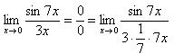
It is necessary to calculate the limit
As you can see, this limit is very similar to the first remarkable one, but this is not entirely true. In general, if you notice sin in the limit, then you should immediately think about whether it is possible to use the first remarkable limit.
According to our rule No. 1, we substitute zero instead of x:
We get uncertainty.
Now let's try to organize the first wonderful limit ourselves. To do this, let's do a simple combination:
So we organize the numerator and denominator to highlight 7x. Now the familiar remarkable limit has already appeared. It is advisable to highlight it when deciding:
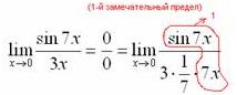
Let's substitute the solution of the first wonderful example and we get:
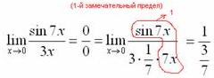
Simplifying the fraction:
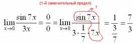
Answer: 7/3.
As you can see, everything is very simple.
Looks like ![]() , where e = 2.718281828... is an irrational number.
, where e = 2.718281828... is an irrational number.
Various functions may be present instead of the variable x, the main thing is that they tend to .
It is necessary to calculate the limit
Here we see the presence of a degree under the sign of a limit, which means it is possible to use a second remarkable limit.
As always, we will use rule No. 1 - substitute x instead of:
It can be seen that at x the base of the degree is , and the exponent is 4x > , i.e. we obtain an uncertainty of the form:
![]()
Let's use the second wonderful limit to reveal our uncertainty, but first we need to organize it. As you can see, we need to achieve presence in the indicator, for which we raise the base to the power of 3x, and at the same time to the power of 1/3x, so that the expression does not change:
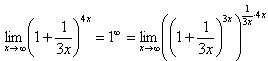
Don't forget to highlight our wonderful limit:
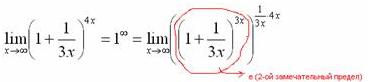
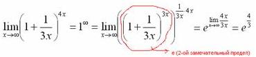
That's what they really are wonderful limits!
If you still have any questions about the first and second wonderful limits, then feel free to ask them in the comments.
We will answer everyone as much as possible.
You can also work with a teacher on this topic.
We are pleased to offer you the services of selecting a qualified tutor in your city. Our partners will quickly select a good teacher for you on favorable terms.
Not enough information? - You can !
You can write math calculations in notepads. It is much more pleasant to write individually in notebooks with a logo (http://www.blocnot.ru).