Derivative calculations are often found in Unified State Exam assignments. This page contains a list of formulas for finding derivatives.

Rules of differentiation

1. (k⋅ f(x))′=k⋅ f ′(x).
2. (f(x)+g(x))′=f′(x)+g′(x).
3. (f(x)⋅ g(x))′=f′(x)⋅ g(x)+f(x)⋅ g′(x).
4. Derivative of a complex function. If y=F(u), and u=u(x), then the function y=f(x)=F(u(x)) is called a complex function of x. Equal to y′(x)=Fu′⋅ ux′.
5. Derivative of an implicit function. The function y=f(x) is called an implicit function defined by the relation F(x,y)=0 if F(x,f(x))≡0.
6. Derivative of the inverse function. If g(f(x))=x, then the function g(x) is called the inverse function of the function y=f(x).
7. Derivative of a parametrically defined function. Let x and y be specified as functions of the variable t: x=x(t), y=y(t). They say that y=y(x) parametrically given function on the interval x∈ (a;b), if on this interval the equation x=x(t) can be expressed as t=t(x) and the function y=y(t(x))=y(x) can be defined.
8. Derivative of a power-exponential function. Found by taking logarithms to the base of the natural logarithm.

We advise you to save the link, as this table may be needed many times.

We present without proof the formulas for the derivatives of the basic elementary functions:

1. Power function: (x n)` =nx n -1 .

2. Exponential function: (a x)` =a x lna(in particular, (e x)` = e x).

3. Logarithmic function: (in particular, (lnx)` = 1/x).

4. Trigonometric functions:

(cosх)` = -sinx

(tgх)` = 1/cos 2 x

(ctgх)` = -1/sin 2 x

5. Inverse trigonometric functions:

It can be proven that to differentiate a power-exponential function, it is necessary to use the formula for the derivative of a complex function twice, namely, differentiate it as a complex power function, and as a complex exponential, and add the results: (f(x)  (x))` =(x)*f(x)  (x)-1 *f(x)` +f(x)  ( x) *lnf(x)*(x)`.

Higher order derivatives

Since the derivative of a function is itself a function, it can also have a derivative. The concept of a derivative, which was discussed above, refers to a first-order derivative.

Derivativen-th order is called the derivative of the (n- 1)th order derivative. For example, f``(x) = (f`(x))` - second order derivative (or second derivative), f```(x) = (f``(x))` - third order derivative (or third derivative), etc. Sometimes Roman Arabic numerals in parentheses are used to denote higher-order derivatives, for example, f (5) (x) or f (V) (x) for a fifth-order derivative.

The physical meaning of derivatives of higher orders is determined in the same way as for the first derivative: each of them represents the rate of change of the derivative of the previous order. For example, the second derivative represents the rate of change of the first, i.e. speed speed. For rectilinear motion, it means the acceleration of a point at a moment in time.

Elasticity function

Elasticity function E x (y) is the limit of the ratio of the relative increment of the function y to the relative increment of the argument x as the latter tends to zero:
.

The elasticity of a function shows approximately how many percent the function y = f(x) will change when the independent variable x changes by 1%.

In an economic sense, the difference between this indicator and the derivative is that the derivative has units of measurement, and therefore its value depends on the units in which the variables are measured. For example, if the dependence of production volume on time is expressed in tons and months, respectively, then the derivative will show the marginal increase in volume in tons per month; if we measure these indicators, say, in kilograms and days, then both the function itself and its derivative will be different. Elasticity is essentially a dimensionless quantity (measured in percentages or shares) and therefore does not depend on the scale of indicators.

Basic theorems on differentiable functions and their applications

Fermat's theorem. If a function differentiable on an interval reaches its greatest or minimum value at an internal point of this interval, then the derivative of the function at this point is zero.

No proof.

The geometric meaning of Fermat's theorem is that at the point of the largest or smallest value achieved inside the interval, the tangent to the graph of the function is parallel to the abscissa axis (Figure 3.3).

Rolle's theorem. Let the function y =f(x) satisfy the following conditions:

2) differentiable on the interval (a, b);

3) at the ends of the segment takes equal values, i.e. f(a) =f(b).

Then there is at least one point inside the segment at which the derivative of the function is equal to zero.

No proof.

The geometric meaning of Rolle's theorem is that there is at least one point at which the tangent to the graph of the function will be parallel to the abscissa axis (for example, in Figure 3.4 there are two such points).

If f(a) =f(b) = 0, then Rolle’s theorem can be formulated differently: between two consecutive zeros of the differentiable function there is at least one zero of the derivative.

Rolle's theorem is a special case of Lagrange's theorem.

Lagrange's theorem. Let the function y =f(x) satisfy the following conditions:

1) continuous on the interval [a, b];

2) differentiable on the interval (a, b).

Then inside the segment there is at least one such point c, at which the derivative is equal to the quotient of the function increment divided by the argument increment on this segment:
.

No proof.

To understand the physical meaning of Lagrange’s theorem, we note that
is nothing more than the average rate of change of the function over the entire interval [a, b]. Thus, the theorem states that inside the segment there is at least one point at which the “instantaneous” rate of change of the function is equal to the average rate of its change over the entire segment.

The geometric meaning of Lagrange's theorem is illustrated in Figure 3.5. Note that the expression
represents the angular coefficient of the straight line on which the chord AB lies. The theorem states that on the graph of a function there will be at least one point at which the tangent to it will be parallel to this chord (i.e., the slope of the tangent - the derivative - will be the same).

Corollary: if the derivative of a function is equal to zero on a certain interval, then the function is identically constant on this interval.

In fact, let us take the interval . According to Lagrange's theorem, in this interval there is a point c for which
. Hence f(a) – f(x) = f `(с)(a – x) = 0; f(x) = f(a) = const.

L'Hopital's rule. The limit of the ratio of two infinitesimal or infinitely large functions is equal to the limit of the ratio of their derivatives (finite or infinite), if the latter exists in the indicated sense.

In other words, if there is uncertainty of the form
, That
.

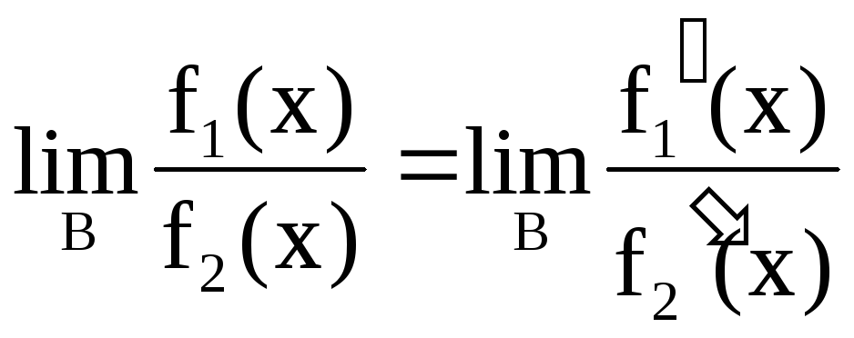No proof.

The application of L'Hopital's rule to find limits will be discussed in practical classes.

Sufficient condition for an increase (decrease) of a function. If the derivative of a differentiable function is positive (negative) within a certain interval, then the function increases (decreases) on this interval.

Proof. Consider two values ​​x 1 and x 2 from this interval (let x 2 > x 1). By Lagrand's theorem on [x 1, x 2] there is a point c at which
. Hence f(x 2) –f(x 1) =f`(c)(x 2 –x 1). Then for f`(c) > 0 the left side of the inequality is positive, i.e. f(x 2) >f(x 1), and the function is increasing. Whenf`(c)< 0 left side inequality is negative, i.e. f(x 2)

The theorem has been proven.

Geometric interpretation of the condition for the monotonicity of a function: if the tangents to the curve in a certain interval are directed at acute angles to the abscissa axis, then the function increases, and if at obtuse angles, then it decreases (see Figure 3.6).

Note: the necessary condition for monotonicity is weaker. If a function increases (decreases) over a certain interval, then the derivative is non-negative (non-positive) on this interval (that is, at individual points the derivative of a monotonic function can be equal to zero).

Prove formulas 3 and 5 yourself.

BASIC RULES OF DIFFERENTIATION

Using the general method of finding the derivative using the limit, one can obtain the simplest differentiation formulas. Let u=u(x),v=v(x)– two differentiable functions of a variable x.

Prove formulas 1 and 2 yourself.

Proof of Formula 3.

Let y = u(x) + v(x). For argument value x+Δ x we have y(x+Δ x)=u(x+Δ x) + v(x+Δ x).

Δ y=y(x+Δ x) – y(x) = u(x+Δ x) + v(x+Δ x) – u(x) – v(x) = Δ u +Δ v.

Hence,

Proof of formula 4.

Let y=u(x)·v(x). Then y(x+Δ x)=u(x+Δ x)· v(x+Δ x), That's why

Δ y=u(x+Δ x)· v(x+Δ x) – u(x)· v(x).

Note that since each of the functions u And v differentiable at the point x, then they are continuous at this point, which means u(x+Δ x)→u(x), v(x+Δ x)→v(x), at Δ x→0.

Therefore we can write

Based on this property, one can obtain a rule for differentiating the product of any number of functions.

Let, for example, y=u·v·w. Then,

y " = u "·( v w) + u·( v·w) " = u "· v·w + u·( v"·w+ v·w ") = u "· v·w + u· v"·w+ u·v·w ".

Proof of formula 5.

Let . Then

In the proof we used the fact that v(x+Δ x)→v(x) at Δ x→0.

Examples.

THEOREM ON THE DERIVATIVE OF COMPLEX FUNCTION

Let y = f(u), A u= u(x). We get the function y depending on the argument x: y = f(u(x)). The last function is called a function of a function or complex function.

Function definition domain y = f(u(x)) is either the entire domain of definition of the function u=u(x) or that part in which the values ​​are determined u, not leaving the domain of definition of the function y= f(u).

The function-from-function operation can be performed not just once, but any number of times.

Let us establish a rule for differentiating a complex function.

Theorem. If the function u= u(x) has at some point x 0 derivative and takes the value at this point u 0 = u(x 0), and the function y=f(u) has at the point u 0 derivative y" u = f "(u 0), then a complex function y = f(u(x)) at the specified point x 0 also has a derivative, which is equal to y" x = f "(u 0)· u "(x 0), where instead of u the expression must be substituted u= u(x).

Thus, the derivative of a complex function is equal to the product of the derivative of a given function with respect to the intermediate argument u to the derivative of the intermediate argument with respect to x.

Proof. For a fixed value X 0 we will have u 0 =u(x 0), at 0 =f(u 0 ). For a new argument value x 0+Δ x:

Δ u= u(x 0 + Δ x) – u(x 0), Δ y=f(u 0+Δ u) – f(u 0).

Because u– differentiable at a point x 0, That u– is continuous at this point. Therefore, at Δ x→0 Δ u→0. Similarly for Δ u→0 Δ y→0.

By condition . From this relation, using the definition of the limit, we obtain (at Δ u→0)

where α→0 at Δ u→0, and, consequently, at Δ x→0.

Let us rewrite this equality as:

Δ y=y" uΔ u+α·Δ u.

The resulting equality is also valid for Δ u=0 for arbitrary α, since it turns into the identity 0=0. At Δ u=0 we will assume α=0. Let us divide all terms of the resulting equality by Δ x

.

By condition . Therefore, passing to the limit at Δ x→0, we get y" x = y"u·u" x. The theorem has been proven.

So, to differentiate a complex function y = f(u(x)), you need to take the derivative of the "external" function f, treating its argument simply as a variable, and multiply by the derivative of the "internal" function with respect to the independent variable.

If the function y=f(x) can be represented in the form y=f(u), u=u(v), v=v(x), then finding the derivative y " x is carried out by sequential application of the previous theorem.

According to the proven rule, we have y" x = y" u u"x. Applying the same theorem for u"x we get, i.e.

y" x = y" x u" v v" x = f"u( u)· u" v ( v)· v" x ( x).

Examples.

THE CONCEPT OF AN INVERSE FUNCTION

Let's start with an example. Consider the function y= x 3. We will consider the equality y= x 3 as an equation relative x. This is the equation for each value at defines a single value x: . Geometrically, this means that every straight line parallel to the axis Ox intersects the graph of a function y= x 3 only at one point. Therefore we can consider x as a function of y. A function is called the inverse of a function y= x 3.

Before moving on to the general case, we introduce definitions.

Function y = f(x) called increasing on a certain segment, if the larger value of the argument x from this segment corresponds higher value functions, i.e. If x 2 >x 1, then f(x 2 ) > f(x 1 ).

The function is called similarly decreasing, if a smaller value of the argument corresponds to a larger value of the function, i.e. If X 2 < X 1, then f(x 2 ) > f(x 1 ).

So, let's be given an increasing or decreasing function y=f(x), defined on some interval [ a; b]. For definiteness, we will consider an increasing function (for a decreasing one everything is similar).

Consider two different values X 1 and X 2. Let y 1 =f(x 1 ), y 2 =f(x 2 ). From the definition of an increasing function it follows that if x 1 <x 2, then at 1 <at 2. Therefore, two different values X 1 and X 2 corresponds to two different function values at 1 and at 2. The opposite is also true, i.e. If at 1 <at 2, then from the definition of an increasing function it follows that x 1 <x 2. Those. again two different values at 1 and at 2 corresponds to two different values x 1 and x 2. Thus, between the values x and their corresponding values y a one-to-one correspondence is established, i.e. the equation y=f(x) for each y(taken from the range of the function y=f(x)) defines a single value x, and we can say that x there is some argument function y: x= g(y).

This function is called reverse for function y=f(x). Obviously, the function y=f(x) is the inverse of the function x=g(y).

Note that the inverse function x=g(y) found by solving the equation y=f(x) relatively X.

Example. Let the function be given y= e x . This function increases at –∞< x <+∞. Она имеет обратную функцию x= log y. Domain of inverse function 0< y < + ∞.

Let's make a few comments.

Note 1. If an increasing (or decreasing) function y=f(x) is continuous on the interval [ a; b], and f(a)=c, f(b)=d, then the inverse function is defined and continuous on the interval [ c; d].

Note 2. If the function y=f(x) is neither increasing nor decreasing on a certain interval, then it can have several inverse functions.

Example. Function y=x2 defined at –∞<x<+∞. Она не является ни возрастающей, ни убывающей и не имеет обратной функции. Однако, если мы рассмотриминтервал 0≤x<+∞, то здесь функция является возрастающей и обратной для нее будет . На интервале – ∞ <x≤ 0 function – decreases and its inverse.

Note 3. If the functions y=f(x) And x=g(y) are mutually inverse, then they express the same relationship between variables x And y. Therefore, the graph of both is the same curve. But if we denote the argument of the inverse function again by x, and the function through y and plot them in the same coordinate system, we will get two different graphs. It is easy to notice that the graphs will be symmetrical with respect to the bisector of the 1st coordinate angle.

THEOREM ON THE DERIVATIVE INVERSE FUNCTION

Let us prove a theorem that allows us to find the derivative of the function y=f(x), knowing the derivative of the inverse function.

Theorem. If for the function y=f(x) there is an inverse function x=g(y), which at some point at 0 has a derivative g "(v 0), nonzero, then at the corresponding point x 0=g(x 0) function y=f(x) has a derivative f "(x 0), equal to , i.e. the formula is correct.

Proof. Because x=g(y) differentiable at the point y 0, That x=g(y) is continuous at this point, so the function y=f(x) continuous at a point x 0=g(y 0). Therefore, at Δ x→0 Δ y→0.

Let's show that .

Let . Then, by the property of the limit . Let us pass in this equality to the limit at Δ y→0. Then Δ x→0 and α(Δx)→0, i.e. .

Hence,

,

Q.E.D.

This formula can be written in the form .

Let's look at the application of this theorem using examples.

The operation of finding the derivative is called differentiation.

As a result of solving problems of finding derivatives of the simplest (and not very simple) functions by defining the derivative as the limit of the ratio of the increment to the increment of the argument, a table of derivatives and precisely defined rules of differentiation appeared. The first to work in the field of finding derivatives were Isaac Newton (1643-1727) and Gottfried Wilhelm Leibniz (1646-1716).

Therefore, in our time, to find the derivative of any function, you do not need to calculate the above-mentioned limit of the ratio of the increment of the function to the increment of the argument, but you only need to use the table of derivatives and the rules of differentiation. The following algorithm is suitable for finding the derivative.

To find the derivative, you need an expression under the prime sign break down simple functions into components and determine what actions (product, sum, quotient) these functions are related. Next, we find the derivatives of elementary functions in the table of derivatives, and the formulas for the derivatives of the product, sum and quotient - in the rules of differentiation. The derivative table and differentiation rules are given after the first two examples.

Example 1. Find the derivative of a function

Solution. From the rules of differentiation we find out that the derivative of a sum of functions is the sum of derivatives of functions, i.e.

From the table of derivatives we find out that the derivative of "x" is equal to one, and the derivative of sine is equal to cosine. We substitute these values ​​into the sum of derivatives and find the derivative required by the condition of the problem:

Example 2. Find the derivative of a function

Solution. We differentiate as a derivative of a sum in which the second term has a constant factor; it can be taken out of the sign of the derivative:

If questions still arise about where something comes from, they are usually cleared up after familiarizing yourself with the table of derivatives and the simplest rules of differentiation. We are moving on to them right now.

Table of derivatives of simple functions

1. Derivative of a constant (number). Any number (1, 2, 5, 200...) that is in the function expression. Always equal to zero. This is very important to remember, as it is required very often
2. Derivative of the independent variable. Most often "X". Always equal to one. This is also important to remember for a long time
3. Derivative of degree. When solving problems, you need to convert non-square roots into powers.
4. Derivative of a variable to the power -1
5. Derivative of square root
6. Derivative of sine
7. Derivative of cosine
8. Derivative of tangent
9. Derivative of cotangent
10. Derivative of arcsine
11. Derivative of arccosine
12. Derivative of arctangent
13. Derivative of arc cotangent
14. Derivative of the natural logarithm
15. Derivative of a logarithmic function
16. Derivative of the exponent
17. Derivative of an exponential function

Rules of differentiation

1. Derivative of a sum or difference
2. Derivative of the product
2a. Derivative of an expression multiplied by a constant factor
3. Derivative of the quotient
4. Derivative of a complex function

Rule 1.If the functions

are differentiable at some point, then the functions are differentiable at the same point

and

those. the derivative of an algebraic sum of functions is equal to the algebraic sum of the derivatives of these functions.

Consequence. If two differentiable functions differ by a constant term, then their derivatives are equal, i.e.

Rule 2.If the functions

are differentiable at some point, then their product is differentiable at the same point

and

those. The derivative of the product of two functions is equal to the sum of the products of each of these functions and the derivative of the other.

Corollary 1. The constant factor can be taken out of the sign of the derivative:

Corollary 2. The derivative of the product of several differentiable functions is equal to the sum of the products of the derivative of each factor and all the others.

For example, for three multipliers:

Rule 3.If the functions

differentiable at some point And , then at this point their quotient is also differentiableu/v , and

those. the derivative of the quotient of two functions is equal to a fraction, the numerator of which is the difference between the products of the denominator and the derivative of the numerator and the numerator and the derivative of the denominator, and the denominator is the square of the former numerator.

Where to look for things on other pages

When finding the derivative of a product and a quotient in real problems, it is always necessary to apply several differentiation rules at once, so there are more examples on these derivatives in the article"Derivative of the product and quotient of functions".

Comment. You should not confuse a constant (that is, a number) as a term in a sum and as a constant factor! In the case of a term, its derivative is equal to zero, and in the case of a constant factor, it is taken out of the sign of the derivatives. This is a typical mistake that occurs at the initial stage of studying derivatives, but as the average student solves several one- and two-part examples, he no longer makes this mistake.

And if, when differentiating a product or quotient, you have a term u"v, in which u- a number, for example, 2 or 5, that is, a constant, then the derivative of this number will be equal to zero and, therefore, the entire term will be equal to zero (this case is discussed in example 10).

Another common mistake is mechanically solving the derivative of a complex function as the derivative of a simple function. That's why derivative of a complex function a separate article is devoted. But first we will learn to find derivatives of simple functions.

Along the way, you can’t do without transforming expressions. To do this, you may need to open the manual in new windows. Actions with powers and roots And Operations with fractions .

If you are looking for solutions to derivatives of fractions with powers and roots, that is, when the function looks like , then follow the lesson “Derivative of sums of fractions with powers and roots.”

If you have a task like , then you will take the lesson “Derivatives of simple trigonometric functions”.

Step-by-step examples - how to find the derivative

Example 3. Find the derivative of a function

Solution. We define the parts of the function expression: the entire expression represents a product, and its factors are sums, in the second of which one of the terms contains a constant factor. We apply the product differentiation rule: the derivative of the product of two functions is equal to the sum of the products of each of these functions by the derivative of the other:

Next, we apply the rule of differentiation of the sum: the derivative of the algebraic sum of functions is equal to the algebraic sum of the derivatives of these functions. In our case, in each sum the second term has a minus sign. In each sum we see both an independent variable, the derivative of which is equal to one, and a constant (number), the derivative of which is equal to zero. So, “X” turns into one, and minus 5 turns into zero. In the second expression, "x" is multiplied by 2, so we multiply two by the same unit as the derivative of "x". We obtain the following derivative values:

We substitute the found derivatives into the sum of products and obtain the derivative of the entire function required by the condition of the problem:

And you can check the solution to the derivative problem on.

Example 4. Find the derivative of a function

Solution. We are required to find the derivative of the quotient. We apply the formula for differentiating the quotient: the derivative of the quotient of two functions is equal to a fraction, the numerator of which is the difference between the products of the denominator and the derivative of the numerator and the numerator and the derivative of the denominator, and the denominator is the square of the former numerator. We get:

We have already found the derivative of the factors in the numerator in example 2. Let us also not forget that the product, which is the second factor in the numerator in the current example, is taken with a minus sign:

If you are looking for solutions to problems in which you need to find the derivative of a function, where there is a continuous pile of roots and powers, such as, for example, , then welcome to class "Derivative of sums of fractions with powers and roots" .

If you need to learn more about the derivatives of sines, cosines, tangents and other trigonometric functions, that is, when the function looks like , then a lesson for you "Derivatives of simple trigonometric functions" .

Example 5. Find the derivative of a function

Solution. In this function we see a product, one of the factors of which is the square root of the independent variable, the derivative of which we familiarized ourselves with in the table of derivatives. Using the rule for differentiating the product and the tabular value of the derivative of the square root, we obtain:

You can check the solution to the derivative problem at online derivatives calculator .

Example 6. Find the derivative of a function

Solution. In this function we see a quotient whose dividend is the square root of the independent variable. Using the rule of differentiation of quotients, which we repeated and applied in example 4, and the tabulated value of the derivative of the square root, we obtain:

To get rid of a fraction in the numerator, multiply the numerator and denominator by .

We present a summary table for convenience and clarity when studying the topic.

Constanty = C Power function y = x p (x p) " = p x p - 1	Exponential functiony = ax (a x) " = a x ln a In particular, whena = ewe have y = e x (e x) " = e x
Logarithmic function (log a x) " = 1 x ln a In particular, whena = ewe have y = logx (ln x) " = 1 x	Trigonometric functions (sin x) " = cos x (cos x) " = - sin x (t g x) " = 1 cos 2 x (c t g x) " = - 1 sin 2 x
Inverse trigonometric functions (a r c sin x) " = 1 1 - x 2 (a r c cos x) " = - 1 1 - x 2 (a r c t g x) " = 1 1 + x 2 (a r c c t g x) " = - 1 1 + x 2	Hyperbolic functions (s h x) " = c h x (c h x) " = s h x (t h x) " = 1 c h 2 x (c t h x) " = - 1 s h 2 x

Let us analyze how the formulas of the specified table were obtained or, in other words, we will prove the derivation of derivative formulas for each type of function.

Derivative of a constant

Evidence 1

In order to derive this formula, we take as a basis the definition of the derivative of a function at a point. We use x 0 = x, where x takes the value of any real number, or, in other words, x is any number from the domain of the function f (x) = C. Let's write down the limit of the ratio of the increment of a function to the increment of the argument as ∆ x → 0:

lim ∆ x → 0 ∆ f (x) ∆ x = lim ∆ x → 0 C - C ∆ x = lim ∆ x → 0 0 ∆ x = 0

Please note that the expression 0 ∆ x falls under the limit sign. It is not the uncertainty “zero divided by zero,” since the numerator does not contain an infinitesimal value, but precisely zero. In other words, the increment of a constant function is always zero.

So, the derivative of the constant function f (x) = C is equal to zero throughout the entire domain of definition.

Example 1

The constant functions are given:

f 1 (x) = 3, f 2 (x) = a, a ∈ R, f 3 (x) = 4. 13 7 22 , f 4 (x) = 0 , f 5 (x) = - 8 7

Solution

Let us describe the given conditions. In the first function we see the derivative of the natural number 3. In the following example, you need to take the derivative of A, Where A- any real number. The third example gives us the derivative of the irrational number 4. 13 7 22, the fourth is the derivative of zero (zero is an integer). Finally, in the fifth case we have the derivative of the rational fraction - 8 7.

Answer: derivatives of given functions are zero for any real x(over the entire definition area)

f 1 " (x) = (3) " = 0 , f 2 " (x) = (a) " = 0 , a ∈ R , f 3 " (x) = 4 . 13 7 22 " = 0 , f 4 " (x) = 0 " = 0 , f 5 " (x) = - 8 7 " = 0

Derivative of a power function

Let's move on to the power function and the formula for its derivative, which has the form: (x p) " = p x p - 1, where the exponent p is any real number.

Evidence 2

Here is the proof of the formula when the exponent is a natural number: p = 1, 2, 3, …

We again rely on the definition of a derivative. Let's write down the limit of the ratio of the increment of a power function to the increment of the argument:

(x p) " = lim ∆ x → 0 = ∆ (x p) ∆ x = lim ∆ x → 0 (x + ∆ x) p - x p ∆ x

To simplify the expression in the numerator, we use Newton’s binomial formula:

(x + ∆ x) p - x p = C p 0 + x p + C p 1 · x p - 1 · ∆ x + C p 2 · x p - 2 · (∆ x) 2 + . . . + + C p p - 1 x (∆ x) p - 1 + C p p (∆ x) p - x p = = C p 1 x p - 1 ∆ x + C p 2 x p - 2 (∆ x) 2 + . . . + C p p - 1 x (∆ x) p - 1 + C p p (∆ x) p

Thus:

(x p) " = lim ∆ x → 0 ∆ (x p) ∆ x = lim ∆ x → 0 (x + ∆ x) p - x p ∆ x = = lim ∆ x → 0 (C p 1 x p - 1 ∆ x + C p 2 x p - 2 (∆ x) 2 + ... + C p p - 1 x (∆ x) p - 1 + C p p (∆ x) p) ∆ x = = lim ∆ x → 0 (C p 1 x p - 1 + C p 2 x p - 2 ∆ x + . . + C p p - 1 x (∆ x) p - 2 + C p p (∆ x) p - 1) = = C p 1 · x p - 1 + 0 + 0 + . . . + 0 = p ! 1 ! · (p - 1) ! · x p - 1 = p · x p - 1

Thus, we have proven the formula for the derivative of a power function when the exponent is a natural number.

Evidence 3

To provide evidence for the case when p- any real number other than zero, we use the logarithmic derivative (here we should understand the difference from the derivative of a logarithmic function). To have a more complete understanding, it is advisable to study the derivative of a logarithmic function and further understand the derivative of an implicit function and the derivative of a complex function.

Let's consider two cases: when x positive and when x negative.

So x > 0. Then: x p > 0 . Let us logarithm the equality y = x p to base e and apply the property of the logarithm:

y = x p ln y = ln x p ln y = p · ln x

At this stage, we have obtained an implicitly specified function. Let's define its derivative:

(ln y) " = (p · ln x) 1 y · y " = p · 1 x ⇒ y " = p · y x = p · x p x = p · x p - 1

Now we consider the case when x – a negative number.

If the indicator p is an even number, then the power function is defined for x< 0 , причем является четной: y (x) = - y ((- x) p) " = - p · (- x) p - 1 · (- x) " = = p · (- x) p - 1 = p · x p - 1

Then x p< 0 и возможно составить доказательство, используя логарифмическую производную.

If p is an odd number, then the power function is defined for x< 0 , причем является нечетной: y (x) = - y (- x) = - (- x) p . Тогда x p < 0 , а значит логарифмическую производную задействовать нельзя. В такой ситуации возможно взять за основу доказательства правила дифференцирования и правило нахождения производной сложной функции:

y " (x) = (- (- x) p) " = - ((- x) p) " = - p · (- x) p - 1 · (- x) " = = p · (- x) p - 1 = p x p - 1

The last transition is possible due to the fact that if p is an odd number, then p - 1 either an even number or zero (for p = 1), therefore, for negative x the equality (- x) p - 1 = x p - 1 is true.

So, we have proven the formula for the derivative of a power function for any real p.

Example 2

Functions given:

f 1 (x) = 1 x 2 3 , f 2 (x) = x 2 - 1 4 , f 3 (x) = 1 x log 7 12

Determine their derivatives.

Solution

We transform some of the given functions into tabular form y = x p , based on the properties of the degree, and then use the formula:

f 1 (x) = 1 x 2 3 = x - 2 3 ⇒ f 1 " (x) = - 2 3 x - 2 3 - 1 = - 2 3 x - 5 3 f 2 " (x) = x 2 - 1 4 = 2 - 1 4 x 2 - 1 4 - 1 = 2 - 1 4 x 2 - 5 4 f 3 (x) = 1 x log 7 12 = x - log 7 12 ⇒ f 3" ( x) = - log 7 12 x - log 7 12 - 1 = - log 7 12 x - log 7 12 - log 7 7 = - log 7 12 x - log 7 84

Derivative of an exponential function

Proof 4

Let us derive the derivative formula using the definition as a basis:

(a x) " = lim ∆ x → 0 a x + ∆ x - a x ∆ x = lim ∆ x → 0 a x (a ∆ x - 1) ∆ x = a x lim ∆ x → 0 a ∆ x - 1 ∆ x = 0 0

We got uncertainty. To expand it, let's write a new variable z = a ∆ x - 1 (z → 0 as ∆ x → 0). In this case, a ∆ x = z + 1 ⇒ ∆ x = log a (z + 1) = ln (z + 1) ln a . For the last transition, the formula for transition to a new logarithm base was used.

Let us substitute into the original limit:

(a x) " = a x · lim ∆ x → 0 a ∆ x - 1 ∆ x = a x · ln a · lim ∆ x → 0 1 1 z · ln (z + 1) = = a x · ln a · lim ∆ x → 0 1 ln (z + 1) 1 z = a x · ln a · 1 ln lim ∆ x → 0 (z + 1) 1 z

Let us remember the second remarkable limit and then we obtain the formula for the derivative of the exponential function:

(a x) " = a x · ln a · 1 ln lim z → 0 (z + 1) 1 z = a x · ln a · 1 ln e = a x · ln a

Example 3

The exponential functions are given:

f 1 (x) = 2 3 x , f 2 (x) = 5 3 x , f 3 (x) = 1 (e) x

It is necessary to find their derivatives.

Solution

We use the formula for the derivative of the exponential function and the properties of the logarithm:

f 1 " (x) = 2 3 x " = 2 3 x ln 2 3 = 2 3 x (ln 2 - ln 3) f 2 " (x) = 5 3 x " = 5 3 x ln 5 1 3 = 1 3 5 3 x ln 5 f 3 " (x) = 1 (e) x " = 1 e x " = 1 e x ln 1 e = 1 e x ln e - 1 = - 1 e x

Derivative of a logarithmic function

Evidence 5

Let us provide a proof of the formula for the derivative of a logarithmic function for any x in the domain of definition and any permissible values ​​of the base a of the logarithm. Based on the definition of derivative, we get:

(log a x) " = lim ∆ x → 0 log a (x + ∆ x) - log a x ∆ x = lim ∆ x → 0 log a x + ∆ x x ∆ x = = lim ∆ x → 0 1 ∆ x log a 1 + ∆ x x = lim ∆ x → 0 log a 1 + ∆ x x 1 ∆ x = = lim ∆ x → 0 log a 1 + ∆ x x 1 ∆ x · x x = lim ∆ x → 0 1 x · log a 1 + ∆ x x x ∆ x = = 1 x · log a lim ∆ x → 0 1 + ∆ x x x ∆ x = 1 x · log a e = 1 x · ln e ln a = 1 x · ln a

From the indicated chain of equalities it is clear that the transformations were based on the property of the logarithm. The equality lim ∆ x → 0 1 + ∆ x x x ∆ x = e is true in accordance with the second remarkable limit.

Example 4

Logarithmic functions are given:

f 1 (x) = log ln 3 x , f 2 (x) = ln x

It is necessary to calculate their derivatives.

Solution

Let's apply the derived formula:

f 1 " (x) = (log ln 3 x) " = 1 x · ln (ln 3) ; f 2 " (x) = (ln x) " = 1 x ln e = 1 x

So, the derivative of the natural logarithm is one divided by x.

Derivatives of trigonometric functions

Proof 6

Let's use some trigonometric formulas and the first wonderful limit to derive the formula for the derivative of a trigonometric function.

According to the definition of the derivative of the sine function, we get:

(sin x) " = lim ∆ x → 0 sin (x + ∆ x) - sin x ∆ x

The formula for the difference of sines will allow us to perform the following actions:

(sin x) " = lim ∆ x → 0 sin (x + ∆ x) - sin x ∆ x = = lim ∆ x → 0 2 sin x + ∆ x - x 2 cos x + ∆ x + x 2 ∆ x = = lim ∆ x → 0 sin ∆ x 2 · cos x + ∆ x 2 ∆ x 2 = = cos x + 0 2 · lim ∆ x → 0 sin ∆ x 2 ∆ x 2

Finally, we use the first wonderful limit:

sin " x = cos x + 0 2 · lim ∆ x → 0 sin ∆ x 2 ∆ x 2 = cos x

So, the derivative of the function sin x will cos x.

We will also prove the formula for the derivative of the cosine:

cos " x = lim ∆ x → 0 cos (x + ∆ x) - cos x ∆ x = = lim ∆ x → 0 - 2 sin x + ∆ x - x 2 sin x + ∆ x + x 2 ∆ x = = - lim ∆ x → 0 sin ∆ x 2 sin x + ∆ x 2 ∆ x 2 = = - sin x + 0 2 lim ∆ x → 0 sin ∆ x 2 ∆ x 2 = - sin x

Those. the derivative of the cos x function will be – sin x.

We derive the formulas for the derivatives of tangent and cotangent based on the rules of differentiation:

t g " x = sin x cos x " = sin " x · cos x - sin x · cos " x cos 2 x = = cos x · cos x - sin x · (- sin x) cos 2 x = sin 2 x + cos 2 x cos 2 x = 1 cos 2 x c t g " x = cos x sin x " = cos " x · sin x - cos x · sin " x sin 2 x = = - sin x · sin x - cos x · cos x sin 2 x = - sin 2 x + cos 2 x sin 2 x = - 1 sin 2 x

Derivatives of inverse trigonometric functions

The section on the derivative of inverse functions provides comprehensive information on the proof of the formulas for the derivatives of arcsine, arccosine, arctangent and arccotangent, so we will not duplicate the material here.

Derivatives of hyperbolic functions

Evidence 7

We can derive the formulas for the derivatives of the hyperbolic sine, cosine, tangent and cotangent using the differentiation rule and the formula for the derivative of the exponential function:

s h " x = e x - e - x 2 " = 1 2 e x " - e - x " = = 1 2 e x - - e - x = e x + e - x 2 = c h x c h " x = e x + e - x 2 " = 1 2 e x " + e - x " = = 1 2 e x + - e - x = e x - e - x 2 = s h x t h " x = s h x c h x " = s h " x · c h x - s h x · c h " x c h 2 x = c h 2 x - s h 2 x c h 2 x = 1 c h 2 x c t h " x = c h x s h x " = c h " x · s h x - c h x · s h " x s h 2 x = s h 2 x - c h 2 x s h 2 x = - 1 s h 2 x

If you notice an error in the text, please highlight it and press Ctrl+Enter