As is known, random variable called variable quantity, which can take one or another value depending on the case. Random variables are denoted by capital letters of the Latin alphabet (X, Y, Z), and their values are denoted by corresponding lowercase letters (x, y, z). Random variables are divided into discontinuous (discrete) and continuous.
Discrete random variable called random value, taking only a finite or infinite (countable) set of values with certain non-zero probabilities.
Distribution law of a discrete random variable is a function that connects the values of a random variable with their corresponding probabilities. The distribution law can be specified in one of the following ways.
1 . The distribution law can be given by the table:
where λ>0, k = 0, 1, 2, … .
V) by using distribution function F(x) , which determines for each value x the probability that the random variable X will take a value less than x, i.e. F(x) = P(X< x).
Properties of the function F(x)
3 . The distribution law can be specified graphically – distribution polygon (polygon) (see problem 3).
Note that to solve some problems it is not necessary to know the distribution law. In some cases, it is enough to know one or more numbers that reflect the most important features distribution law. This can be a number that has the meaning of the “average value” of a random variable, or a number showing the average size of the deviation of a random variable from its mean value. Numbers of this kind are called numerical characteristics of a random variable.
Basic numerical characteristics discrete random variable :
- Mathematical expectation
(average value) of a discrete random variable M(X)=Σ x i p i.
For binomial distribution M(X)=np, for Poisson distribution M(X)=λ - Dispersion
discrete random variable D(X)=M2 or D(X) = M(X 2)− 2. The difference X–M(X) is called the deviation of a random variable from its mathematical expectation.
For binomial distribution D(X)=npq, for Poisson distribution D(X)=λ - Standard deviation (standard deviation) σ(X)=√D(X).
Examples of solving problems on the topic “The law of distribution of a discrete random variable”
Task 1.
1000 lottery tickets were issued: 5 of them will win 500 rubles, 10 will win 100 rubles, 20 will win 50 rubles, 50 will win 10 rubles. Determine the law of probability distribution of the random variable X - winnings per ticket.
Solution. According to the conditions of the problem, the following values of the random variable X are possible: 0, 10, 50, 100 and 500.
The number of tickets without winning is 1000 – (5+10+20+50) = 915, then P(X=0) = 915/1000 = 0.915.
Similarly, we find all other probabilities: P(X=0) = 50/1000=0.05, P(X=50) = 20/1000=0.02, P(X=100) = 10/1000=0.01 , P(X=500) = 5/1000=0.005. Let us present the resulting law in the form of a table:
We'll find expected value values X: M(X) = 1*1/6 + 2*1/6 + 3*1/6 + 4*1/6 + 5*1/6 + 6*1/6 = (1+2+3 +4+5+6)/6 = 21/6 = 3.5
Task 3.
The device consists of three independently operating elements. The probability of failure of each element in one experiment is 0.1. Draw up a distribution law for the number of failed elements in one experiment, construct a distribution polygon. Find the distribution function F(x) and plot it. Find the mathematical expectation, variance and standard deviation of a discrete random variable.
Solution. 1. The discrete random variable X=(the number of failed elements in one experiment) has the following possible values: x 1 =0 (none of the device elements failed), x 2 =1 (one element failed), x 3 =2 (two elements failed) and x 4 =3 (three elements failed).
Failures of elements are independent of each other, the probabilities of failure of each element are equal, therefore it is applicable Bernoulli's formula
. Considering that, according to the condition, n=3, p=0.1, q=1-p=0.9, we determine the probabilities of the values:
P 3 (0) = C 3 0 p 0 q 3-0 = q 3 = 0.9 3 = 0.729;
P 3 (1) = C 3 1 p 1 q 3-1 = 3*0.1*0.9 2 = 0.243;
P 3 (2) = C 3 2 p 2 q 3-2 = 3*0.1 2 *0.9 = 0.027;
P 3 (3) = C 3 3 p 3 q 3-3 = p 3 =0.1 3 = 0.001;
Check: ∑p i = 0.729+0.243+0.027+0.001=1.
Thus, the desired binomial distribution law of X has the form:
We plot the possible values of x i along the abscissa axis, and the corresponding probabilities p i along the ordinate axis. Let's construct points M 1 (0; 0.729), M 2 (1; 0.243), M 3 (2; 0.027), M 4 (3; 0.001). By connecting these points with straight line segments, we obtain the desired distribution polygon.
3. Let's find the distribution function F(x) = Р(Х
For x ≤ 0 we have F(x) = Р(Х<0) = 0;for 0< x ≤1 имеем F(x) = Р(Х<1) = Р(Х = 0) = 0,729;
for 1< x ≤ 2 F(x) = Р(Х<2) = Р(Х=0) + Р(Х=1) =0,729+ 0,243 = 0,972;
for 2< x ≤ 3 F(x) = Р(Х<3) = Р(Х = 0) + Р(Х = 1) + Р(Х = 2) = 0,972+0,027 = 0,999;
for x > 3 there will be F(x) = 1, because the event is reliable.
 |
Graph of function F(x)
4.
For binomial distribution X:
- mathematical expectation M(X) = np = 3*0.1 = 0.3;
- variance D(X) = npq = 3*0.1*0.9 = 0.27;
- standard deviation σ(X) = √D(X) = √0.27 ≈ 0.52.
Numerical characteristics of continuous random variables. Let a continuous random variable X be specified by the distribution function f(x)
Let a continuous random variable X be specified by the distribution function f(x). Let us assume that all possible values of the random variable belong to the segment [ a,b].
Definition. Mathematical expectation a continuous random variable X, the possible values of which belong to the segment , is called a definite integral
If possible values of a random variable are considered on the entire numerical axis, then the mathematical expectation is found by the formula:

In this case, of course, it is assumed that the improper integral converges.
Definition. Variance of a continuous random variable is the mathematical expectation of the square of its deviation.

By analogy with the variance of a discrete random variable, to practically calculate the variance, the formula is used:

Definition. Standard deviation called the square root of the variance.
![]()
Definition. Fashion M 0 of a discrete random variable is called its most probable value. For a continuous random variable, mode is the value of the random variable at which the distribution density has a maximum.
![]()
If the distribution polygon for a discrete random variable or the distribution curve for a continuous random variable has two or more maxima, then such a distribution is called bimodal or multimodal. If a distribution has a minimum but no maximum, then it is called antimodal.
Definition. Median M D of a random variable X is its value relative to which it is equally probable that a larger or smaller value of the random variable will be obtained.
Geometrically, the median is the abscissa of the point at which the area limited by the distribution curve is divided in half. Note that if the distribution is unimodal, then the mode and median coincide with the mathematical expectation.
Definition. The starting moment order k random variable X is the mathematical expectation of the value X k.
For a discrete random variable: .
![]() .
.
The initial moment of the first order is equal to the mathematical expectation.
Definition. Central moment order k random variable X is the mathematical expectation of the value
![]()
For a discrete random variable: ![]() .
.
For a continuous random variable: ![]() .
.
The first order central moment is always zero, and the second order central moment is equal to the dispersion. The third-order central moment characterizes the asymmetry of the distribution.
Definition. The ratio of the central moment of the third order to the standard deviation to the third power is called asymmetry coefficient.
Definition. To characterize the peakedness and flatness of the distribution, a quantity called excess.
In addition to the quantities considered, the so-called absolute moments are also used:
Absolute starting moment: . Absolute central point: ![]() . The absolute central moment of the first order is called arithmetic mean deviation.
. The absolute central moment of the first order is called arithmetic mean deviation.
Example. For the example discussed above, determine the mathematical expectation and variance of the random variable X.

Example. There are 6 white and 4 black balls in an urn. A ball is removed from it five times in a row, and each time the removed ball is returned back and the balls are mixed. Taking the number of extracted white balls as a random variable X, draw up a distribution law for this value, determine its mathematical expectation and dispersion.
Because the balls in each experiment are returned back and mixed, then the tests can be considered independent (the result of the previous experiment does not affect the probability of the occurrence or non-occurrence of an event in another experiment).
Thus, the probability of a white ball appearing in each experiment is constant and equal to
Thus, as a result of five consecutive trials, the white ball may not appear at all, or appear once, twice, three, four or five times. To draw up a distribution law, you need to find the probabilities of each of these events.
1) The white ball did not appear at all:
2) The white ball appeared once:
3) The white ball will appear twice: ![]() .
.
Unlike a discrete random variable, continuous random variables cannot be specified in the form of a table of its distribution law since it is impossible to list and write out all its values in a certain sequence. One possible way to specify a continuous random variable is to use a distribution function.
DEFINITION. The distribution function is a function that determines the probability that a random variable will take the value that is represented on the number axis by a point lying to the left of point x, i.e.
Sometimes instead of the term “Distribution function” the term “Integral function” is used.
Properties of the distribution function:
1. The values of the distribution function belong to the segment: 0F(x)1
2. F(x) is a non-decreasing function, i.e. F(x 2)F(x 1), if x 2 >x 1
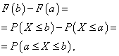
Corollary 1. The probability that a random variable will take a value contained in the interval (a,b) is equal to the increment of the distribution function over this interval:
P(aX
Example 9. Random variable X is given by the distribution function:

Find the probability that as a result of the test X will take a value belonging to the interval (0;2): P(0 Solution: Since on the interval (0;2) by condition, F(x)=x/4+1/4, then F(2)-F(0)=(2/4+1/4)-(0 /4+1/4)=1/2. So P(0 Corollary 2. The probability that a continuous random variable X will take one specific value is zero. Corollary 3. If possible values of a random variable belong to the interval (a;b), then: 1) F(x)=0 for xa; 2) F(x)=1 at xb. The graph of the distribution function is located in the band limited by the straight lines y=0, y=1 (first property). As x increases in the interval (a;b), which contains all possible values of the random variable, the graph “rises up”. At xa, the ordinates of the graph are equal to zero; at xb the ordinates of the graph are equal to one: Example 10. A discrete random variable X is given by a distribution table: Find the distribution function and plot it. DEFINITION: The probability distribution density of a continuous random variable X is the function f(x) - the first derivative of the distribution function F(x): f(x)=F"(x) From this definition it follows that the distribution function is an antiderivative of the distribution density. Theorem. The probability that a continuous random variable X will take a value belonging to the interval (a;b) is equal to a certain integral of the distribution density, taken in the range from a to b: Properties of probability density distribution: 1. The probability density is a non-negative function: f(x)0. Example 11. The probability distribution density of a random variable X is given Solution: Required probability: Let us extend the definition of numerical characteristics of discrete quantities to continuous quantities. Let a continuous random variable X be specified by the distribution density f(x). DEFINITION. The mathematical expectation of a continuous random variable X, the possible values of which belong to the segment , is called a definite integral: M(x)=xf(x)dx (9) If possible values belong to the entire Ox axis, then: M(x)=xf(x)dx (10) The mode M 0 (X) of a continuous random variable X is its possible value to which the local maximum of the distribution density corresponds. The median M e (X) of a continuous random variable X is its possible value, which is determined by the equality: P(X e (X))=P(X>M e (X)) DEFINITION. The variance of a continuous random variable is the mathematical expectation of the square of its deviation. If possible values of X belong to the segment , then: D(x)= 2 f(x)dx (11) If the possible values belong to the entire x-axis, then. Examples of solving problems on the topic “Random variables”.
Task 1
. There are 100 tickets issued for the lottery. One winning of 50 USD was drawn. and ten wins of 10 USD each. Find the law of distribution of the value X - the cost of possible winnings. Solution. Possible values for X: x 1
= 0; x 2
= 10 and x 3
= 50. Since there are 89 “empty” tickets, then p 1
= 0.89, probability of winning $10. (10 tickets) – p 2
= 0.10 and to win 50 USD -p 3
= 0.01. Thus: 0,89
0,10
0,01
Easy to control: . Task 2.
The probability that the buyer has read the product advertisement in advance is 0.6 (p = 0.6). Selective control of the quality of advertising is carried out by surveying buyers before the first one who has studied the advertising in advance. Draw up a distribution series for the number of buyers surveyed. Solution. According to the conditions of the problem, p = 0.6. From: q=1 -p = 0.4. Substituting these values, we get: and construct a distribution series: p i 0,24
Task 3.
A computer consists of three independently working elements: the system unit, the monitor and the keyboard. With a single sharp increase in voltage, the probability of failure of each element is 0.1. Based on the Bernoulli distribution, draw up a distribution law for the number of failed elements during a power surge in the network. Solution. Let's consider Bernoulli distribution(or binomial): the probability that n tests, event A will appear exactly k once: q n p n IN Let's return to the task. Possible values for X (number of failures): x 0 =0 – none of the elements failed; x 1 =1 – failure of one element; x 2 =2 – failure of two elements; x 3 =3 – failure of all elements. Since, by condition, p = 0.1, then q = 1 – p = 0.9. Using Bernoulli's formula, we get , ,
, .
Control: . Therefore, the required distribution law: 0,729
0,243
0,027
0,001
Problem 4. 5000 rounds produced. Probability that one cartridge is defective Solution. Applicable Poisson distribution: This distribution is used to determine the probability that, for very large number of tests (mass tests), in each of which the probability of event A is very small, event A will occur k times: Here n = 5000, p = 0.0002, k = 3. We find , then the desired probability: Problem 5. When firing until the first hit with hit probability p
= 0.6 when firing, you need to find the probability that a hit will occur on the third shot. Solution. Let us apply a geometric distribution: let independent trials be carried out, in each of which event A has a probability of occurrence p (and non-occurrence q = 1 – p). The test ends as soon as event A occurs. Under such conditions, the probability that event A will occur on the kth trial is determined by the formula: . Here p = 0.6; q = 1 – 0.6 = 0.4;k = 3. Therefore, . Problem 6. Let the law of distribution of a random variable X be given: Find the mathematical expectation. Solution. . Note that the probabilistic meaning of the mathematical expectation is the average value of a random variable. Problem 7. Find the variance of the random variable X with the following distribution law: Solution. Here
.
Distribution law for the squared value of X 2
:
X 2
Required variance: . Dispersion characterizes the measure of deviation (dispersion) of a random variable from its mathematical expectation. Problem 8. Let a random variable be given by the distribution: 10m Find its numerical characteristics. Solution: m, m 2
,
M 2
, m. About the random variable X we can say either: its mathematical expectation is 6.4 m with a variance of 13.04 m 2
, or – its mathematical expectation is 6.4 m with a deviation of m. The second formulation is obviously more clear. Task 9.
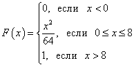
Random value X given by the distribution function: Find the probability that as a result of the test the value X will take the value contained in the interval Solution. The probability that X will take a value from a given interval is equal to the increment of the integral function in this interval, i.e. . In our case and , therefore Task 10.
Discrete random variable X is given by the distribution law: Find the distribution function F(x ) and plot it. Solution. Since the distribution function, at ; at ; at ; at ; Relevant chart: Problem 11. Continuous random variable X given by the differential distribution function: Find the hit probability X per interval Solution. Note that this is a special case of the exponential distribution law. Let's use the formula: Task 12.
Find the numerical characteristics of a discrete random variable X specified by the distribution law: –5
X2: X 2 .
,
Where The values of this function are found using a table. In our case: . From the table we find: , therefore: Random variable
is a variable that can take on certain values depending on various circumstances, and random variable is called continuous
, if it can take any value from any limited or unlimited interval. For a continuous random variable, it is impossible to indicate all possible values, so we designate intervals of these values that are associated with certain probabilities. Examples of continuous random variables include: the diameter of a part being ground to a given size, the height of a person, the flight range of a projectile, etc. Since for continuous random variables the function F(x), Unlike discrete random variables, has no jumps anywhere, then the probability of any individual value of a continuous random variable is zero. This means that for a continuous random variable it makes no sense to talk about the probability distribution between its values: each of them has zero probability. However, in a sense, among the values of a continuous random variable there are “more and less probable”. For example, hardly anyone would doubt that the value of a random variable - the height of a randomly encountered person - 170 cm - is more likely than 220 cm, although both values can occur in practice. As a distribution law that makes sense only for continuous random variables, the concept of distribution density or probability density is introduced. Let's approach it by comparing the meaning of the distribution function for a continuous random variable and for a discrete random variable. So, the distribution function of a random variable (both discrete and continuous) or integral function is called a function that determines the probability that the value of a random variable X less than or equal to the limit value X. For a discrete random variable at the points of its values x1
, x 2
, ..., x i,... masses of probabilities are concentrated p1
, p 2
, ..., p i,..., and the sum of all masses is equal to 1. Let us transfer this interpretation to the case of a continuous random variable. Let's imagine that a mass equal to 1 is not concentrated at individual points, but is continuously “smeared” along the abscissa axis Oh with some uneven density. Probability of a random variable falling into any area Δ x will be interpreted as the mass per section, and the average density at that section as the ratio of mass to length. We have just introduced an important concept in probability theory: distribution density. Probability density f(x) of a continuous random variable is the derivative of its distribution function: Knowing the density function, you can find the probability that the value of a continuous random variable belongs to the closed interval [ a; b]: the probability that a continuous random variable X will take any value from the interval [ a; b], is equal to a certain integral of its probability density ranging from a before b: In this case, the general formula of the function F(x) probability distribution of a continuous random variable, which can be used if the density function is known f(x)
: The probability density graph of a continuous random variable is called its distribution curve (figure below). Area of a figure (shaded in the figure) bounded by a curve, straight lines drawn from points a And b perpendicular to the x-axis, and the axis Oh, graphically displays the probability that the value of a continuous random variable X is within the range of a before b. 1. The probability that a random variable will take any value from the interval (and the area of the figure that is limited by the graph of the function f(x) and axis Oh) is equal to one: 2. The probability density function cannot take negative values: and outside the existence of the distribution its value is zero Distribution density f(x), as well as the distribution function F(x), is one of the forms of the distribution law, but unlike the distribution function, it is not universal: the distribution density exists only for continuous random variables. Let us mention the two most important types of distribution of a continuous random variable in practice. If the distribution density function f(x) continuous random variable in some finite interval [ a; b] takes a constant value C, and outside the interval takes a value equal to zero, then this the distribution is called uniform . If the graph of the distribution density function is symmetrical about the center, the average values are concentrated near the center, and moving away from the center those more different from the average are collected (the graph of the function resembles a section of a bell), then this distribution is called normal . Example 1. The probability distribution function of a continuous random variable is known: Find function f(x) probability density of a continuous random variable. Construct graphs of both functions. Find the probability that a continuous random variable will take any value in the interval from 4 to 8: . Solution. We obtain the probability density function by finding the derivative of the probability distribution function: Graph of a function F(x) - parabola: Graph of a function f(x) - straight: Let's find the probability that a continuous random variable will take any value in the range from 4 to 8: Example 2. The probability density function of a continuous random variable is given as: Calculate coefficient C. Find function F(x) probability distribution of a continuous random variable. Construct graphs of both functions. Find the probability that a continuous random variable will take any value in the range from 0 to 5: . Solution. Coefficient C we find, using property 1 of the probability density function: Thus, the probability density function of a continuous random variable is: By integrating, we find the function F(x) probability distributions. If x < 0
, то
F(x) = 0 . If 0< x < 10
, то x> 10, then F(x) = 1
. Thus, the complete record of the probability distribution function is: Graph of a function f(x)
: Graph of a function F(x)
: Let's find the probability that a continuous random variable will take any value in the range from 0 to 5: Example 3. Probability density of a continuous random variable X is given by the equality , and . Find coefficient A, the probability that a continuous random variable X will take any value from the interval ]0, 5[, the distribution function of a continuous random variable X. Solution. By condition we arrive at equality Therefore, , from where . So, Now we find the probability that a continuous random variable X will take any value from the interval ]0, 5[: Now we get the distribution function of this random variable: Example 4. Find the probability density of a continuous random variable X, which takes only non-negative values, and its distribution function
The following limit relations are valid:
Picture 1X
1
4
8
P
0.3
0.1
0.6
Solution: The distribution function can be written analytically as follows:

Figure-2![]() (8)
(8)
2. The definite integral from -∞ to +∞ of the probability density of a continuous random variable is equal to 1: f(x)dx=1.
3. The definite integral from -∞ to x of the probability density of a continuous random variable is equal to the distribution function of this variable: f(x)dx=F(x)
Find the probability that as a result of the test X will take a value belonging to the interval (0.5;1).
or
D(x)=x 2 f(x)dx- 2 (11*)
![]() , or:
, or:
![]() . What is the probability that there will be exactly 3 defective cartridges in the entire batch?
. What is the probability that there will be exactly 3 defective cartridges in the entire batch? , Where .
 .
.
 .
.
![]() .
.
![]() .
.
![]() For
For ![]() , That
, That
 .
.
 .
.
 – Laplace function.
Distribution function of a continuous random variable and probability density
![]() .
.
![]()
![]() .
.![]() .
.
Properties of the probability density function of a continuous random variable


![]() .
.


![]() .
.

![]() .
.