A function graph is a visual representation of the behavior of a function on a coordinate plane. Graphs help you understand various aspects functions that cannot be determined from the function itself. You can build graphs of many functions, and each of them will be given a specific formula. The graph of any function is built using a specific algorithm (if you have forgotten the exact process of graphing a specific function).
Steps
Graphing a Linear Function
- If the slope is negative, the function is decreasing.
-
From the point where the straight line intersects the Y axis, plot a second point using vertical and horizontal distances. A linear function can be graphed using two points. In our example, the intersection point with the Y axis has coordinates (0.5); From this point, move 2 spaces up and then 1 space to the right. Mark a point; it will have coordinates (1,7). Now you can draw a straight line.
Using a ruler, draw a straight line through two points. To avoid mistakes, find the third point, but in most cases the graph can be plotted using two points. Thus, you have plotted a linear function.
Determine whether the function is linear. The linear function is given by a formula of the form F (x) = k x + b (\displaystyle F(x)=kx+b) or y = k x + b (\displaystyle y=kx+b)(for example, ), and its graph is a straight line. Thus, the formula includes one variable and one constant (constant) without any exponents, root signs, or the like. If a function of a similar type is given, it is quite simple to plot a graph of such a function. Here are other examples linear functions:
Use a constant to mark a point on the Y axis. The constant (b) is the “y” coordinate of the point where the graph intersects the Y axis. That is, it is a point whose “x” coordinate is equal to 0. Thus, if x = 0 is substituted into the formula, then y = b (constant). In our example y = 2 x + 5 (\displaystyle y=2x+5) the constant is equal to 5, that is, the point of intersection with the Y axis has coordinates (0.5). Plot this point on the coordinate plane.
Find the slope of the line. It is equal to the multiplier of the variable. In our example y = 2 x + 5 (\displaystyle y=2x+5) with the variable “x” there is a factor of 2; thus, the slope coefficient is equal to 2. The slope coefficient determines the angle of inclination of the straight line to the X axis, that is, the greater the slope coefficient, the faster the function increases or decreases.
Write the slope as a fraction. The angular coefficient is equal to the tangent of the angle of inclination, that is, the ratio of the vertical distance (between two points on a straight line) to the horizontal distance (between the same points). In our example, the slope is 2, so we can state that the vertical distance is 2 and the horizontal distance is 1. Write this as a fraction: 2 1 (\displaystyle (\frac (2)(1))).
Graphing a Complex Function
-
Find the coordinates of several points and plot them on the coordinate plane. Simply select several x values and plug them into the function to find the corresponding y values. Then plot the points on the coordinate plane. How more complex function, the more points you need to find and plot. In most cases, substitute x = -1; x = 0; x = 1, but if the function is complex, find three points on each side of the origin.
- In case of function y = 5 x 2 + 6 (\displaystyle y=5x^(2)+6) plug in the following x values: -1, 0, 1, -2, 2, -10, 10. You will get a sufficient number of points.
- Choose your x values wisely. In our example, it is easy to understand that the negative sign does not matter: the value of “y” at x = 10 and at x = -10 will be the same.
-
- If you don't know what to do, start with function substitution different meanings"x" to find the "y" values (and therefore the coordinates of the points). Theoretically, a graph of a function can be constructed using only this method (if, of course, one substitutes an infinite variety of “x” values).
Find the zeros of the function. The zeros of a function are the values of the x variable where y = 0, that is, these are the points where the graph intersects the X-axis. Keep in mind that not all functions have zeros, but they are the first step in the process of graphing any function. To find the zeros of a function, equate it to zero. For example:
Find and mark the horizontal asymptotes. An asymptote is a line that the graph of a function approaches but never intersects (that is, in this region the function is not defined, for example, when dividing by 0). Mark the asymptote with a dotted line. If the variable "x" is in the denominator of a fraction (for example, y = 1 4 − x 2 (\displaystyle y=(\frac (1)(4-x^(2))))), set the denominator to zero and find “x”. In the obtained values of the variable “x” the function is not defined (in our example, draw dotted lines through x = 2 and x = -2), because you cannot divide by 0. But asymptotes exist not only in cases where the function contains a fractional expression. Therefore it is recommended to use common sense:
1. Fractional linear function and its graph
A function of the form y = P(x) / Q(x), where P(x) and Q(x) are polynomials, is called a fractional rational function.
With the concept rational numbers you probably already know each other. Likewise rational functions are functions that can be represented as the quotient of two polynomials.
If a fractional rational function is the quotient of two linear functions - polynomials of the first degree, i.e. function of the form
y = (ax + b) / (cx + d), then it is called fractional linear.
Note that in the function y = (ax + b) / (cx + d), c ≠ 0 (otherwise the function becomes linear y = ax/d + b/d) and that a/c ≠ b/d (otherwise the function is constant ). The linear fractional function is defined for all real numbers except x = -d/c. Graphs of fractional linear functions do not differ in shape from the graph y = 1/x you know. A curve that is a graph of the function y = 1/x is called hyperbole. With an unlimited increase in x in absolute value, the function y = 1/x decreases unlimited in absolute value and both branches of the graph approach the abscissa: the right one approaches from above, and the left one from below. The lines to which the branches of a hyperbola approach are called its asymptotes.
Example 1.
y = (2x + 1) / (x – 3).
Solution.
Let's select the whole part: (2x + 1) / (x – 3) = 2 + 7/(x – 3).
Now it is easy to see that the graph of this function is obtained from the graph of the function y = 1/x by the following transformations: shift by 3 unit segments to the right, stretching along the Oy axis 7 times and shifting by 2 unit segments upward.
Any fraction y = (ax + b) / (cx + d) can be written in a similar way, highlighting the “integer part”. Consequently, the graphs of all fractional linear functions are hyperbolas, shifted in various ways along coordinate axes and stretched along the Oy axis.
To construct a graph of any arbitrary fractional-linear function, it is not at all necessary to transform the fraction defining this function. Since we know that the graph is a hyperbola, it will be enough to find the straight lines to which its branches approach - the asymptotes of the hyperbola x = -d/c and y = a/c.
Example 2.
Find the asymptotes of the graph of the function y = (3x + 5)/(2x + 2).
Solution.
The function is not defined, at x = -1. This means that the straight line x = -1 serves as a vertical asymptote. To find the horizontal asymptote, let’s find out what the values of the function y(x) approach when the argument x increases in absolute value.
To do this, divide the numerator and denominator of the fraction by x:
y = (3 + 5/x) / (2 + 2/x).
As x → ∞ the fraction will tend to 3/2. This means that the horizontal asymptote is the straight line y = 3/2.
Example 3.
Graph the function y = (2x + 1)/(x + 1).
Solution.
Let’s select the “whole part” of the fraction:
(2x + 1) / (x + 1) = (2x + 2 – 1) / (x + 1) = 2(x + 1) / (x + 1) – 1/(x + 1) =
2 – 1/(x + 1).
Now it is easy to see that the graph of this function is obtained from the graph of the function y = 1/x by the following transformations: a shift by 1 unit to the left, a symmetrical display with respect to Ox and a shift by 2 unit segments up along the Oy axis.
Domain D(y) = (-∞; -1)ᴗ(-1; +∞).
Range of values E(y) = (-∞; 2)ᴗ(2; +∞).
Intersection points with axes: c Oy: (0; 1); c Ox: (-1/2; 0). The function increases at each interval of the domain of definition.
Answer: Figure 1.
2. Fractional rational function
Consider a fractional rational function of the form y = P(x) / Q(x), where P(x) and Q(x) are polynomials of degree higher than first.
Examples of such rational functions:
y = (x 3 – 5x + 6) / (x 7 – 6) or y = (x – 2) 2 (x + 1) / (x 2 + 3).
If the function y = P(x) / Q(x) represents the quotient of two polynomials of degree higher than the first, then its graph will, as a rule, be more complex, and it can sometimes be difficult to construct it accurately, with all the details. However, it is often enough to use techniques similar to those we have already introduced above.
Let the fraction be a proper fraction (n< m). Известно, что любую несократимую рациональную дробь можно представить, и притом единственным образом, в виде суммы конечного числа элементарных дробей, вид которых определяется разложением знаменателя дроби Q(x) в произведение действительных сомножителей:
P(x)/Q(x) = A 1 /(x – K 1) m1 + A 2 /(x – K 1) m1-1 + … + A m1 /(x – K 1) + …+
L 1 /(x – K s) ms + L 2 /(x – K s) ms-1 + … + L ms /(x – K s) + …+
+ (B 1 x + C 1) / (x 2 +p 1 x + q 1) m1 + … + (B m1 x + C m1) / (x 2 +p 1 x + q 1) + …+
+ (M 1 x + N 1) / (x 2 +p t x + q t) m1 + … + (M m1 x + N m1) / (x 2 +p t x + q t).
Obviously, the graph of a fractional rational function can be obtained as the sum of graphs of elementary fractions.
Plotting graphs of fractional rational functions
Let's consider several ways to construct graphs of a fractional rational function.
Example 4.
Draw a graph of the function y = 1/x 2 .
Solution.
We use the graph of the function y = x 2 to construct a graph of y = 1/x 2 and use the technique of “dividing” the graphs.
Domain D(y) = (-∞; 0)ᴗ(0; +∞).
Range of values E(y) = (0; +∞).
There are no points of intersection with the axes. The function is even. Increases for all x from the interval (-∞; 0), decreases for x from 0 to +∞.
Answer: Figure 2.
Example 5.
Graph the function y = (x 2 – 4x + 3) / (9 – 3x).
Solution.
Domain D(y) = (-∞; 3)ᴗ(3; +∞).
y = (x 2 – 4x + 3) / (9 – 3x) = (x – 3)(x – 1) / (-3(x – 3)) = -(x – 1)/3 = -x/ 3 + 1/3.
Here we used the technique of factorization, reduction and reduction to a linear function.
Answer: Figure 3.

Example 6.
Graph the function y = (x 2 – 1)/(x 2 + 1).
Solution.
The domain of definition is D(y) = R. Since the function is even, the graph is symmetrical about the ordinate. Before building a graph, let’s transform the expression again, highlighting the whole part:
y = (x 2 – 1)/(x 2 + 1) = 1 – 2/(x 2 + 1).
Note that isolating the integer part in the formula of a fractional rational function is one of the main ones when constructing graphs.
If x → ±∞, then y → 1, i.e. the straight line y = 1 is a horizontal asymptote.
Answer: Figure 4.
Example 7.
Let's consider the function y = x/(x 2 + 1) and try to accurately find its largest value, i.e. the most high point right half of the graph. To accurately construct this graph, today's knowledge is not enough. Obviously, our curve cannot “rise” very high, because the denominator quickly begins to “overtake” the numerator. Let's see if the value of the function can be equal to 1. To do this, we need to solve the equation x 2 + 1 = x, x 2 – x + 1 = 0. This equation has no real roots. This means our assumption is incorrect. To find the most great importance function, you need to find out at what largest A the equation A = x/(x 2 + 1) will have a solution. Let's replace the original equation with a quadratic one: Аx 2 – x + А = 0. This equation has a solution when 1 – 4А 2 ≥ 0. From here we find highest value A = 1/2. 
Answer: Figure 5, max y(x) = ½.
Still have questions? Don't know how to graph functions?
To get help from a tutor, register.
The first lesson is free!
website, when copying material in full or in part, a link to the source is required.
Let us choose a rectangular coordinate system on the plane and plot the values of the argument on the abscissa axis X, and on the ordinate - the values of the function y = f(x).
Function graph y = f(x) is the set of all points whose abscissas belong to the domain of definition of the function, and the ordinates are equal to the corresponding values of the function.
In other words, the graph of the function y = f (x) is the set of all points of the plane, coordinates X, at which satisfy the relation y = f(x).

In Fig. 45 and 46 show graphs of functions y = 2x + 1 And y = x 2 - 2x.
Strictly speaking, one should distinguish between a graph of a function (the exact mathematical definition of which was given above) and a drawn curve, which always gives only a more or less accurate sketch of the graph (and even then, as a rule, not the entire graph, but only its part located in the final parts of the plane). In what follows, however, we will generally say “graph” rather than “graph sketch.”
Using a graph, you can find the value of a function at a point. Namely, if the point x = a belongs to the domain of definition of the function y = f(x), then to find the number f(a)(i.e. the function values at the point x = a) you should do this. It is necessary through the abscissa point x = a draw a straight line parallel to the ordinate axis; this line will intersect the graph of the function y = f(x) at one point; the ordinate of this point will, by virtue of the definition of the graph, be equal to f(a)(Fig. 47).

For example, for the function f(x) = x 2 - 2x using the graph (Fig. 46) we find f(-1) = 3, f(0) = 0, f(1) = -l, f(2) = 0, etc.
A function graph clearly illustrates the behavior and properties of a function. For example, from consideration of Fig. 46 it is clear that the function y = x 2 - 2x accepts positive values at X< 0 and at x > 2, negative - at 0< x < 2; smallest value function y = x 2 - 2x accepts at x = 1.
To graph a function f(x) you need to find all the points of the plane, coordinates X,at which satisfy the equation y = f(x). In most cases, this is impossible to do, since there are an infinite number of such points. Therefore, the graph of the function is depicted approximately - with greater or lesser accuracy. The simplest is the method of plotting a graph using several points. It consists in the fact that the argument X give a finite number of values - say, x 1, x 2, x 3,..., x k and create a table that includes the selected function values.
The table looks like this:
Having compiled such a table, we can outline several points on the graph of the function y = f(x). Then, connecting these points with a smooth line, we get an approximate view of the graph of the function y = f(x).
It should be noted, however, that the multi-point plotting method is very unreliable. In fact, the behavior of the graph between the intended points and its behavior outside the segment between the extreme points taken remains unknown.
Example 1. To graph a function y = f(x) someone compiled a table of argument and function values:
The corresponding five points are shown in Fig. 48.

Based on the location of these points, he concluded that the graph of the function is a straight line (shown in Fig. 48 by the dotted line). Can this conclusion be considered reliable? Unless there are additional considerations to support this conclusion, it can hardly be considered reliable. reliable.
To substantiate our statement, consider the function
![]() .
.
Calculations show that the values of this function at points -2, -1, 0, 1, 2 are exactly described by the table above. However, the graph of this function is not a straight line at all (it is shown in Fig. 49). Another example would be the function y = x + l + sinπx; its meanings are also described in the table above.

These examples show that in its “pure” form the method of plotting a graph using several points is unreliable. Therefore, to plot a graph of a given function, one usually proceeds as follows. First, we study the properties of this function, with the help of which we can build a sketch of the graph. Then, by calculating the values of the function at several points (the choice of which depends on the established properties of the function), the corresponding points of the graph are found. And finally, a curve is drawn through the constructed points using the properties of this function.
We will look at some (the simplest and most frequently used) properties of functions used to find a graph sketch later, but now we will look at some commonly used methods for constructing graphs.
Graph of the function y = |f(x)|.
It is often necessary to plot a function y = |f(x)|, where f(x) - given function. Let us remind you how this is done. A-priory absolute value numbers can be written
![]()
This means that the graph of the function y =|f(x)| can be obtained from the graph, function y = f(x) as follows: all points on the graph of the function y = f(x), whose ordinates are non-negative, should be left unchanged; further, instead of the points of the graph of the function y = f(x) having negative coordinates, you should construct the corresponding points on the graph of the function y = -f(x)(i.e. part of the graph of the function
y = f(x), which lies below the axis X, should be reflected symmetrically about the axis X).

Example 2. Graph the function y = |x|.
Let's take the graph of the function y = x(Fig. 50, a) and part of this graph at X< 0 (lying under the axis X) symmetrically reflected relative to the axis X. As a result, we get a graph of the function y = |x|(Fig. 50, b).
Example 3. Graph the function y = |x 2 - 2x|.

First, let's plot the function y = x 2 - 2x. The graph of this function is a parabola, the branches of which are directed upward, the vertex of the parabola has coordinates (1; -1), its graph intersects the x-axis at points 0 and 2. In the interval (0; 2) the function takes negative values, therefore this part of the graph symmetrically reflected relative to the abscissa axis. Figure 51 shows the graph of the function y = |x 2 -2x|, based on the graph of the function y = x 2 - 2x
Graph of the function y = f(x) + g(x)
Consider the problem of constructing a graph of a function y = f(x) + g(x). if function graphs are given y = f(x) And y = g(x).
Note that the domain of definition of the function y = |f(x) + g(x)| is the set of all those values of x for which both functions y = f(x) and y = g(x) are defined, i.e. this domain of definition is the intersection of the domains of definition, functions f(x) and g(x).
Let the points (x 0 , y 1) And (x 0, y 2) respectively belong to the graphs of functions y = f(x) And y = g(x), i.e. y 1 = f(x 0), y 2 = g(x 0). Then the point (x0;. y1 + y2) belongs to the graph of the function y = f(x) + g(x)(for f(x 0) + g(x 0) = y 1 +y2),. and any point on the graph of the function y = f(x) + g(x) can be obtained this way. Therefore, the graph of the function y = f(x) + g(x) can be obtained from function graphs y = f(x). And y = g(x) replacing each point ( x n, y 1) function graphics y = f(x) dot (x n, y 1 + y 2), Where y 2 = g(x n), i.e. by shifting each point ( x n, y 1) function graph y = f(x) along the axis at by the amount y 1 = g(x n). In this case, only such points are considered X n for which both functions are defined y = f(x) And y = g(x).
This method of plotting a function y = f(x) + g(x) is called addition of graphs of functions y = f(x) And y = g(x)
Example 4. In the figure, a graph of the function was constructed using the method of adding graphs
y = x + sinx.
When plotting a function y = x + sinx we thought that f(x) = x, A g(x) = sinx. To plot the function graph, we select points with abscissas -1.5π, -, -0.5, 0, 0.5,, 1.5, 2. Values f(x) = x, g(x) = sinx, y = x + sinx Let's calculate at the selected points and place the results in the table.
Function $f(x)=|x|$
$|x|$ - module. It is defined as follows: If real number will be non-negative, then the modulus value coincides with the number itself. If it is negative, then the modulus value coincides with the absolute value of the given number.
Mathematically, this can be written as follows:
Example 1
Function $f(x)=[x]$
The function $f\left(x\right)=[x]$ is a function of the integer part of a number. It is found by rounding the number (if it is not an integer itself) “downwards”.
Example: $=2.$
Example 2
Let's explore and build its graph.
- $D\left(f\right)=R$.
- Obviously, this function only accepts integer values, that is, $\E\left(f\right)=Z$
- $f\left(-x\right)=[-x]$. Therefore, this function will be of a general form.
- $(0,0)$ is the only point of intersection with the coordinate axes.
- $f"\left(x\right)=0$
- The function has discontinuity points (function jumps) for all $x\in Z$.
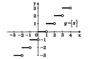
Figure 2.
Function $f\left(x\right)=\(x\)$
The function $f\left(x\right)=\(x\)$ is a function of the fractional part of a number. It is found by “discarding” the integer part of this number.
Example 3
Let's explore and plot the function

Function $f(x)=sign(x)$
The function $f\left(x\right)=sign(x)$ is a signum function. This function shows which sign a real number has. If the number is negative, then the function has the value $-1$. If the number is positive, then the function equals one. If the number is zero, the function value will also take on a zero value.