Inequalities are relations of the form a › b, where a and b are expressions containing at least one variable. Inequalities can be strict - ‹, › and non-strict - ≥, ≤.
Trigonometric inequalities are expressions of the form: F(x) › a, F(x) ‹ a, F(x) ≤ a, F(x) ≥ a, in which F(x) is represented by one or more trigonometric functions.
An example of the simplest trigonometric inequality is: sin x ‹ 1/2. It is customary to solve such problems graphically; two methods have been developed for this.
Method 1 - Solving inequalities by graphing a function
To find an interval that satisfies the conditions inequality sin x ‹ 1/2, you must perform the following steps:
- On coordinate axis construct a sinusoid y = sin x.
- On the same axis, draw a graph of the numerical argument of the inequality, i.e., a straight line passing through the point ½ of the ordinate OY.
- Mark the intersection points of the two graphs.
- Shade the segment that is the solution to the example.
When strict signs are present in an expression, the intersection points are not solutions. Since the smallest positive period of a sinusoid is 2π, we write the answer as follows:
![]()
If the signs of the expression are not strict, then the solution interval must be enclosed in square brackets - . The answer to the problem can also be written as the following inequality: ![]()
Method 2 - Solving trigonometric inequalities using the unit circle
Similar problems can be easily solved using a trigonometric circle. The algorithm for finding answers is very simple:
- First you need to draw a unit circle.
- Then you need to note the value of the arc function of the argument of the right side of the inequality on the arc of the circle.
- It is necessary to draw a straight line passing through the value of the arc function parallel to the abscissa axis (OX).
- After that, all that remains is to select the arc of a circle, which is the set of solutions to the trigonometric inequality.
- Write down the answer in the required form.
Let us analyze the stages of the solution using the example of the inequality sin x › 1/2. Points α and β are marked on the circle - values
![]()
The points of the arc located above α and β are the interval for solving the given inequality.

If you need to solve an example for cos, then the answer arc will be located symmetrically to the OX axis, not OY. You can consider the difference between the solution intervals for sin and cos in the diagrams below in the text.

Graphical solutions for tangent and cotangent inequalities will differ from both sine and cosine. This is due to the properties of functions.

Arctangent and arccotangent are tangents to a trigonometric circle, and the minimum positive period for both functions is π. To quickly and correctly use the second method, you need to remember on which axis the values of sin, cos, tg and ctg are plotted.
The tangent tangent runs parallel to the OY axis. If we plot the value of arctan a on the unit circle, then the second required point will be located in the diagonal quarter. Angles
They are break points for the function, since the graph tends to them, but never reaches them.

In the case of cotangent, the tangent runs parallel to the OX axis, and the function is interrupted at points π and 2π.

Complex trigonometric inequalities
If the argument of the inequality function is represented not just by a variable, but by an entire expression containing an unknown, then we are talking about a complex inequality. The process and procedure for solving it are somewhat different from the methods described above. Suppose we need to find a solution to the following inequality:

The graphical solution involves constructing an ordinary sinusoid y = sin x using arbitrarily selected values of x. Let's calculate a table with coordinates for the control points of the graph:

The result should be a beautiful curve.
To make finding a solution easier, let’s replace the complex function argument

The intersection of two graphs allows us to determine the area of the desired values at which the inequality condition is satisfied.

The found segment is a solution for the variable t:

However, the goal of the task is to find everything possible options unknown x:

Solving the double inequality is quite simple; you need to move π/3 to the extreme parts of the equation and perform the required calculations:

Answer to the task will look like the interval for strict inequality:

Such problems will require students' experience and dexterity in handling trigonometric functions. The more training tasks are solved during the preparation process, the easier and faster the student will find the answer to the question. Unified State Exam question test.
Ministry of Education of the Republic of Belarus
Educational institution
"Gomel State University
named after Francysk Skaryna"
Faculty of Mathematics
Department of Algebra and Geometry
Accepted for defense
Head Department Shemetkov L.A.
Trigonometric equations and inequalities
Course work
Executor:
student of group M-51
CM. Gorsky
Scientific supervisor Ph.D.-M.Sc.,
Senior Lecturer
V.G. Safonov
Gomel 2008
INTRODUCTION
BASIC METHODS FOR SOLVING TRIGONOMETRIC EQUATIONS
Factorization
Solving equations by converting the product of trigonometric functions into a sum
Solving equations using triple argument formulas
Multiplying by some trigonometric function
NON-STANDARD TRIGONOMETRIC EQUATIONS
TRIGONOMETRIC INEQUALITIES
SELECTION OF ROOTS
TASKS FOR INDEPENDENT SOLUTION
CONCLUSION
LIST OF SOURCES USED
In ancient times, trigonometry arose in connection with the needs of astronomy, land surveying and construction, that is, it was purely geometric in nature and represented mainly<<исчисление хорд>>. Over time, some analytical moments began to intersperse into it. In the first half of the 18th century there was a sharp change, after which trigonometry took a new direction and shifted towards mathematical analysis. It was at this time that trigonometric relationships began to be considered as functions.
Trigonometric equations are one of the most difficult topics in a school mathematics course. Trigonometric equations arise when solving problems in planimetry, stereometry, astronomy, physics and other fields. Trigonometric equations and inequalities are found among centralized testing tasks year after year.
The most important difference trigonometric equations from algebraic ones is that in algebraic equations there is a finite number of roots, and in trigonometric ones there is an infinite number, which greatly complicates the selection of roots. Another specific feature of trigonometric equations is the non-unique form of writing the answer.
This thesis is devoted to methods for solving trigonometric equations and inequalities.
The thesis consists of 6 sections.
The first section provides basic theoretical information: definition and properties of trigonometric and inverse trigonometric functions; table of values of trigonometric functions for some arguments; expressing trigonometric functions in terms of other trigonometric functions, which is very important for transforming trigonometric expressions, especially those containing inverse trigonometric functions; except the main ones trigonometric formulas, well known from the school course, formulas are given for simplifying expressions containing inverse trigonometric functions.
The second section outlines the basic methods for solving trigonometric equations. The solution of elementary trigonometric equations, the factorization method, and methods for reducing trigonometric equations to algebraic ones are considered. Due to the fact that solutions to trigonometric equations can be written in several ways, and the form of these solutions does not allow one to immediately determine whether these solutions are the same or different, which may<<сбить с толку>> when solving tests, the general scheme for solving trigonometric equations is considered and the transformation of groups of general solutions of trigonometric equations is considered in detail.
The third section examines non-standard trigonometric equations, the solutions of which are based on the functional approach.
The fourth section discusses trigonometric inequalities. Methods for solving elementary trigonometric inequalities, both on the unit circle and by the graphical method, are discussed in detail. The process of solving non-elementary trigonometric inequalities through elementary inequalities and the method of intervals, already well known to schoolchildren, is described.
The fifth section presents the most difficult tasks: when it is necessary not only to solve a trigonometric equation, but also to select roots from the found roots that satisfy some condition. This section provides solutions to typical root selection tasks. The necessary theoretical information for selecting roots is given: partitioning a set of integers into disjoint subsets, solving equations in integers (diaphantine).
The sixth section presents tasks for independent solution, presented in the form of a test. The 20 test tasks contain the most difficult tasks that can be encountered during centralized testing.
Elementary trigonometric equations
Elementary trigonometric equations are equations of the form , where --- one of the trigonometric functions: , , , .
Elementary trigonometric equations have an infinite number of roots. For example, the following values satisfy the equation: , , , etc. General formula along which all the roots of the equation are found, where , is:
Here it can take any integer values, each of them corresponds to a specific root of the equation; in this formula (as well as in other formulas by which elementary trigonometric equations are solved) are called parameter. They usually write , thereby emphasizing that the parameter can accept any integer values.
Solutions of the equation , where , are found by the formula
The equation is solved using the formula
![]()
and the equation is by the formula
![]()
Let us especially note some special cases of elementary trigonometric equations, when the solution can be written without using general formulas:
![]()
![]()
![]()
![]()
![]()
![]()
![]()
![]()
When solving trigonometric equations, the period of trigonometric functions plays an important role. Therefore, we present two useful theorems:
Theorem If --- the main period of the function, then the number is the main period of the function.
The periods of the functions and are said to be commensurable if there exist integers So what .
Theorem If periodic functions and , have commensurate and , then they have a common period, which is the period of the functions , , .
The theorem states that the period of the function , , , is, and is not necessarily the main period. For example, the main period of the functions and --- , and the main period of their product --- .
Introducing an auxiliary argument
By the standard way of transforming expressions of the form ![]() is the following technique: let --- corner, given by the equalities
is the following technique: let --- corner, given by the equalities ![]() ,
, ![]() . For any, such an angle exists. Thus . If , or , , , in other cases.
. For any, such an angle exists. Thus . If , or , , , in other cases.
Scheme for solving trigonometric equations
The basic scheme that we will follow when solving trigonometric equations is as follows:
solution given equation comes down to solving elementary equations. Solutions --- conversions, factorization, replacement of unknowns. The guiding principle is not to lose your roots. This means that when moving to the next equation(s), we are not afraid of the appearance of extra (extraneous) roots, but only care that each subsequent equation of our “chain” (or a set of equations in the case of branching) is a consequence of the previous one. One of possible methods root selection is a check. Let us immediately note that in the case of trigonometric equations, the difficulties associated with selecting roots and checking, as a rule, increase sharply compared to algebraic equations. After all, we have to check series consisting of infinite number members.
Special mention should be made of the replacement of unknowns when solving trigonometric equations. In most cases, after the necessary replacement, it turns out algebraic equation. Moreover, equations are not so rare that, although they are trigonometric in appearance, essentially they are not, since after the first step --- replacements variables --- turn into algebraic ones, and a return to trigonometry occurs only at the stage of solving elementary trigonometric equations.
Let us remind you once again: the replacement of the unknown should be done at the first opportunity; the resulting equation after the replacement must be solved to the end, including the stage of selecting the roots, and only then returned to the original unknown.
One of the features of trigonometric equations is that the answer can, in many cases, be written in a variety of ways. Even to solve the equation ![]() the answer can be written as follows:
the answer can be written as follows:
1) in the form of two series: ![]() , , ;
, , ;
2) in standard form, which is a combination of the above series: , ;
3) because ![]() , then the answer can be written in the form
, then the answer can be written in the form ![]() , . (In what follows, the presence of the , , or parameter in the response record automatically means that this parameter accepts all possible integer values. Exceptions will be specified.)
, . (In what follows, the presence of the , , or parameter in the response record automatically means that this parameter accepts all possible integer values. Exceptions will be specified.)
Obviously, the three listed cases do not exhaust all the possibilities for writing the answer to the equation under consideration (there are infinitely many of them).
For example, when the equality is true ![]() . Therefore, in the first two cases, if , we can replace by
. Therefore, in the first two cases, if , we can replace by ![]() .
.
Usually the answer is written on the basis of point 2. It is useful to remember the following recommendation: if the work does not end with solving the equation, it is still necessary to conduct research and select roots, then the most convenient form of recording is indicated in point 1. (A similar recommendation should be given for the equation.)
Let's consider an example illustrating what has been said.
Example Solve the equation.
Solution. The most obvious way is the following. This equation breaks down into two: and . Solving each of them and combining the answers obtained, we find .
Another way. Since , then, replacing and using the formulas for reducing the degree. After small transformations we get , from where ![]() .
.
At first glance, the second formula does not have any special advantages over the first. However, if we take, for example, then it turns out that, i.e. the equation has a solution, while the first method leads us to the answer ![]() . "See" and prove equality
. "See" and prove equality ![]() not so easy.
not so easy.
Answer. .
Converting and combining groups of general solutions of trigonometric equations
We will consider an arithmetic progression that extends indefinitely in both directions. The members of this progression can be divided into two groups of members, located to the right and left of a certain member called the central or zero member of the progression.
By fixing one of the terms of an infinite progression with a zero number, we will have to carry out double numbering for all remaining terms: positive for terms located to the right, and negative for terms located to the left of zero.
IN general case, if the difference of the progression is the zero term, the formula for any (th) term of an infinite arithmetic progression is:
Formula transformations for any term of an infinite arithmetic progression
1. If you add or subtract the difference of the progression to the zero term, then the progression will not change, but only the zero term will move, i.e. The numbering of members will change.
2. If the coefficient at variable multiplied by , then this will only result in a rearrangement of the right and left groups of members.
3. If successive terms of an infinite progression
for example, , , ..., , make the central terms of progressions with the same difference equal to:

then a progression and a series of progressions express the same numbers.
Example The row can be replaced by the following three rows: , , .
4. If infinite progressions with the same difference have as central terms numbers that form an arithmetic progression with difference , then these series can be replaced by one progression with difference , and with a central term equal to any of the central terms of these progressions, i.e. If

then these progressions are combined into one:
Example
. . . both are combined into one group, since ![]() .
.
To transform groups that have common solutions into groups that do not have common solutions, these groups are decomposed into groups with a common period, and then try to unite the resulting groups, excluding repeating ones.
Factorization
The factorization method is as follows: if
then every solution of the equation
is the solution to a set of equations
The converse statement is, generally speaking, false: not every solution to the population is a solution to the equation. This is explained by the fact that solutions to individual equations may not be included in the domain of definition of the function.
Example Solve the equation.
Solution. Using the basic trigonometric identity, we represent the equation in the form
Answer.
; ![]() .
.
Converting the sum of trigonometric functions into a product
Example
Solve the equation ![]() .
.
Solution. Applying the formula, we obtain the equivalent equation
![]()
Answer. .
Example Solve the equation.
Solution. In this case, before applying the formulas for the sum of trigonometric functions, you should use the reduction formula ![]() . As a result, we obtain the equivalent equation
. As a result, we obtain the equivalent equation
![]()
Answer.
![]() ,
, ![]() .
.
Solving equations by converting the product of trigonometric functions into a sum
When solving a number of equations, formulas are used.
Example Solve the equation
Solution.
Answer. , .
Example Solve the equation.
Solution. Applying the formula, we obtain an equivalent equation:
Answer. .
Solving equations using reduction formulas
When solving a wide range of trigonometric equations, formulas play a key role.
Example Solve the equation.
Solution. Applying the formula, we obtain an equivalent equation.
Answer. ; .
Solving equations using triple argument formulas
Example Solve the equation.
Solution. Applying the formula, we get the equation
Answer. ; .
Example
Solve the equation ![]() .
.
Solution. Applying the formulas for reducing the degree we get: ![]() . Applying we get:
. Applying we get:
Answer. ; .
Equality of trigonometric functions of the same name
![]()

Example Solve the equation.
Solution.

Answer. , .
Example
Solve the equation ![]() .
.
Solution. Let's transform the equation.
Answer. .
Example It is known that and satisfy the equation
![]()
Find the amount.
Solution. From the equation it follows that
![]()

Answer. .
Let us consider sums of the form
These amounts can be converted into a product by multiplying and dividing them by, then we get

This technique can be used to solve some trigonometric equations, but it should be borne in mind that as a result, extraneous roots may appear. Let us summarize these formulas:


Example Solve the equation.
Solution. It can be seen that the set is a solution to the original equation. Therefore, multiplying the left and right sides of the equation by will not lead to the appearance of extra roots.
We have ![]() .
.
Answer. ; .
Example Solve the equation.
Solution. Let's multiply the left and right sides of the equation by and apply the formulas for converting the product of trigonometric functions into a sum, we get
![]()
This equation is equivalent to the combination of two equations and , whence and .
Since the roots of the equation are not the roots of the equation, we should exclude . This means that in the set it is necessary to exclude .
Answer. And , .
Example
Solve the equation ![]() .
.
Solution. Let's transform the expression:
The equation will be written as:
Answer. .
Reducing trigonometric equations to algebraic ones
Reducible to square
If the equation is of the form
then the replacement leads it to square, since ![]() () And.
() And.
If instead of the term there is , then the required replacement will be .
The equation
comes down to quadratic equation
presentation as ![]() . It is easy to check that for which , are not roots of the equation, and by making the substitution , the equation is reduced to a quadratic one.
. It is easy to check that for which , are not roots of the equation, and by making the substitution , the equation is reduced to a quadratic one.
Example Solve the equation.
Solution. Let's move it to the left side, replace it with , and express it through and .
After simplifications we get: . Divide term by term and make the replacement:
![]()
Returning to , we find ![]() .
.
Equations homogeneous with respect to ,
Consider an equation of the form

where , , , ..., , are real numbers. In each term on the left side of the equation, the degrees of the monomials are equal, that is, the sum of the degrees of sine and cosine is the same and equal. This equation is called homogeneous relative to and , and the number is called homogeneity indicator .
It is clear that if , then the equation will take the form:
![]()
the solutions of which are the values at which , i.e., the numbers , . The second equation written in brackets is also homogeneous, but the degrees are 1 lower.
If , then these numbers are not the roots of the equation.
When we get: , and left side equation (1) takes the value .
So, for , and , therefore we can divide both sides of the equation by . As a result, we get the equation:
which, by substitution, can easily be reduced to algebraic:
Homogeneous equations with homogeneity index 1. When we have the equation .
If , then this equation is equivalent to the equation , , whence , .
Example Solve the equation.
Solution. This equation is homogeneous of the first degree. Divide both parts by we get: , , , .
Answer. .
Example When we get homogeneous equation kind
Solution.
If , then divide both sides of the equation by , we get the equation ![]() , which can be easily reduced to square by substitution:
, which can be easily reduced to square by substitution: ![]() . If
. If ![]() , then the equation has real roots , . The original equation will have two groups of solutions: , , .
, then the equation has real roots , . The original equation will have two groups of solutions: , , .
If ![]() , then the equation has no solutions.
, then the equation has no solutions.
Example Solve the equation.
Solution. This equation homogeneous second degrees. Divide both sides of the equation by , we get: . Let , then , , . , , ; . . .
Answer.
![]() .
.
The equation is reduced to an equation of the form

To do this, it is enough to use the identity ![]()
In particular, the equation is reduced to homogeneous if we replace it with ![]() , then we get an equivalent equation:
, then we get an equivalent equation:
Example Solve the equation.
Solution. Let's transform the equation to a homogeneous one:
Let's divide both sides of the equation by ![]() , we get the equation:
, we get the equation:
![]() Let , then we come to the quadratic equation:
Let , then we come to the quadratic equation: ![]() , ,
, , ![]() ,
, ![]() , .
, .
![]()
Answer.
![]() .
.
Example Solve the equation.
Solution. Let's square both sides of the equation, given that they have positive values: , ,
Let it be, then we get ![]() , , .
, , .
![]()
Answer. .
Equations solved using identities ![]()
It is useful to know the following formulas:
Example Solve the equation.
Solution. Using, we get
![]()
Answer.
![]()
We offer not the formulas themselves, but a method for deriving them:
hence,
Likewise, .
Example
Solve the equation ![]() .
.
Solution. Let's transform the expression:
The equation will be written as:
By accepting, we receive. , . Hence
Answer. .
Universal trigonometric substitution
Trigonometric equation of the form
Where --- rational a function with the help of formulas - , as well as with the help of formulas - can be reduced to a rational equation with respect to the arguments , , , , after which the equation can be reduced to an algebraic rational equation with respect to using the formulas of universal trigonometric substitution


It should be noted that the use of formulas can lead to a narrowing of the OD of the original equation, since it is not defined at the points, so in such cases it is necessary to check whether the angles are the roots of the original equation.
Example Solve the equation.
Solution. According to the conditions of the task. Applying the formulas and making the substitution, we get
from where and therefore .
Equations of the form
Equations of the form , where --- a polynomial, are solved using changes of unknowns

Example Solve the equation.
Solution. Making the replacement and taking into account that , we get
![]()
where , . --- outsider root, because . Roots of the equation ![]() are .
are .
Using feature limitations
In the practice of centralized testing, it is not so rare to encounter equations whose solution is based on the limited functions and . For example:
Example Solve the equation.
Solution. Since , , then the left side does not exceed and is equal to , if
To find values that satisfy both equations, we proceed as follows. Let's solve one of them, then among the found values we will select those that satisfy the other.
Let's start with the second: , . Then , ![]() .
.
It is clear that only for even numbers there will be .
Answer. .
Another idea is realized by solving the following equation:
Example
Solve the equation ![]() .
.
Solution. Let's use the property exponential function: , ![]() .
.
Adding these inequalities term by term we have:
Therefore, the left side of this equation is equal if and only if two equalities hold:
i.e., it can take on the values , , , or it can take on the values , .
Answer. , .
Example
Solve the equation ![]() .
.
Solution., . Hence,  .
.
Answer. .
Example Solve the equation
![]()
Solution. Let us denote , then from the definition of the inverse trigonometric function we have ![]() And
And ![]() .
.
Since, then the inequality follows from the equation, i.e. . Since and , then and . However, that's why.
If and, then. Since it was previously established that , then .
Answer. , .
Example Solve the equation

Solution. The range of acceptable values of the equation is .
First we show that the function
For any, it can only take positive values.
Let's imagine the function as follows: .
Since , then it takes place, i.e. ![]() .
.
Therefore, to prove the inequality, it is necessary to show that ![]() . For this purpose, let us cube both sides of this inequality, then
. For this purpose, let us cube both sides of this inequality, then
The resulting numerical inequality indicates that . If we also take into account that , then the left side of the equation is non-negative.
Let's now look at the right side of the equation.
Because ![]() , That
, That
However, it is known that ![]() . It follows that , i.e. the right side of the equation does not exceed . It was previously proven that the left side of the equation is non-negative, so equality in can only happen if both sides are equal, and this is only possible if .
. It follows that , i.e. the right side of the equation does not exceed . It was previously proven that the left side of the equation is non-negative, so equality in can only happen if both sides are equal, and this is only possible if .
Answer. .
Example Solve the equation
Solution. Let us denote and ![]() . Applying the Cauchy-Bunyakovsky inequality, we obtain . It follows that
. Applying the Cauchy-Bunyakovsky inequality, we obtain . It follows that ![]() . On the other hand, there is
. On the other hand, there is ![]() . Therefore, the equation has no roots.
. Therefore, the equation has no roots.
Answer. .
Example Solve the equation:
Solution. Let's rewrite the equation as:
Answer. .
Functional methods for solving trigonometric and combined equations
Not every equation as a result of transformations can be reduced to an equation of one or another standard form, for which there is a specific solution method. In such cases, it turns out to be useful to use such properties of functions and as monotonicity, boundedness, parity, periodicity, etc. So, if one of the functions decreases and the second increases on the interval, then if the equation has a root on this interval, this root is unique, and then, for example, it can be found by selection. If the function is bounded above, and , and the function is bounded below, and , then the equation is equivalent to the system of equations
Example Solve the equation
![]()
Solution. Let's transform the original equation to the form
![]()
and solve it as a quadratic relative to . Then we get,

Let's solve the first equation of the population. Taking into account the limited nature of the function, we come to the conclusion that the equation can only have a root on the segment. On this interval the function increases, and the function ![]() decreases. Therefore, if this equation has a root, then it is unique. We find by selection.
decreases. Therefore, if this equation has a root, then it is unique. We find by selection.
Answer. .
Example Solve the equation
![]()
Solution. Let and ![]() , then the original equation can be written as a functional equation. Since the function is odd, then . In this case, we get the equation.
, then the original equation can be written as a functional equation. Since the function is odd, then . In this case, we get the equation.
Since , and is monotonic on , the equation is equivalent to the equation, i.e. ![]() , which has a single root.
, which has a single root.
Answer. .
Example
Solve the equation ![]() .
.
Solution. Based on the derivative theorem complex function it is clear that the function ![]() decreasing (function decreasing, increasing, decreasing). From this it is clear that the function
decreasing (function decreasing, increasing, decreasing). From this it is clear that the function ![]() defined on , decreasing. Therefore, this equation has at most one root. Because
defined on , decreasing. Therefore, this equation has at most one root. Because ![]() , That
, That
Answer. .
Example Solve the equation.
Solution. Let's consider the equation on three intervals.
a) Let . Then on this set the original equation is equivalent to the equation . Which has no solutions on the interval, because ![]() , , A . On the interval, the original equation also has no roots, because
, , A . On the interval, the original equation also has no roots, because ![]() , A .
, A .
b) Let . Then on this set the original equation is equivalent to the equation
![]()
whose roots on the interval are the numbers , , , .
c) Let . Then on this set the original equation is equivalent to the equation
![]()
Which has no solutions on the interval, because , and . On the interval, the equation also has no solutions, because ![]() , , A .
, , A .
Answer. , , , .
Symmetry method
The symmetry method is convenient to use when the formulation of the task requires the unique solution of an equation, inequality, system, etc. or an exact indication of the number of solutions. In this case, any symmetry of the given expressions should be detected.
It is also necessary to take into account the variety of different possible types of symmetry.
Equally important is strict adherence to logical stages in reasoning with symmetry.
Typically, symmetry allows us to establish only the necessary conditions, and then we need to check their sufficiency.
Example Find all values of the parameter for which the equation has a unique solution.
Solution. Note that and are even functions, so the left side of the equation is an even function.
So if --- solution equations, that is, also the solution of the equation. If --- the only thing solution to the equation, then necessary , .
We'll select possible values, requiring that it be the root of the equation.
Let us immediately note that other values cannot satisfy the conditions of the problem.
But it is not yet known whether all those selected actually satisfy the conditions of the task.
Adequacy.
1), the equation will take the form ![]() .
.
2), the equation will take the form:
It is obvious that, for everyone and ![]() . Therefore, the last equation is equivalent to the system:
. Therefore, the last equation is equivalent to the system:
Thus, we have proven that for , the equation has a unique solution.
Answer. .
Solution with function exploration
Example Prove that all solutions of the equation
Whole numbers.
Solution. The main period of the original equation is . Therefore, we first examine this equation on the interval.
Let's transform the equation to the form:
![]()
Using a microcalculator we get:
![]()
![]()
If , then from the previous equalities we obtain:
![]()
Having solved the resulting equation, we get: .
The calculations performed make it possible to assume that the roots of the equation belonging to the segment are , and .
Direct testing confirms this hypothesis. Thus, it has been proven that the roots of the equation are only integers , .
Example
Solve the equation ![]() .
.
Solution. Let's find the main period of the equation. The function has a basic period equal to . The main period of the function is . The least common multiple of and is equal to . Therefore, the main period of the equation is . Let .
Obviously, it is a solution to the equation. On the interval. The function is negative. Therefore, other roots of the equation should be sought only on the intervals x and .
Using a microcalculator, we first find the approximate values of the roots of the equation. To do this, we compile a table of function values ![]() on the intervals and ; i.e. on the intervals and .
on the intervals and ; i.e. on the intervals and .
| 0 | 0 | 202,5 | 0,85355342 |
| 3 | -0,00080306 | 207 | 0,6893642 |
| 6 | -0,00119426 | 210 | 0,57635189 |
| 9 | -0,00261932 | 213 | 0,4614465 |
| 12 | -0,00448897 | 216 | 0,34549155 |
| 15 | -0,00667995 | 219 | 0,22934931 |
| 18 | -0,00903692 | 222 | 0,1138931 |
| 21 | -0,01137519 | 225 | 0,00000002 |
| 24 | -0,01312438 | 228 | -0,11145712 |
| 27 | -0,01512438 | 231 | -0,21961736 |
| 30 | -0,01604446 | 234 | -0,32363903 |
| 33 | -0,01597149 | 237 | -0,42270819 |
| 36 | -0,01462203 | 240 | -0,5160445 |
| 39 | -0,01170562 | 243 | -0,60290965 |
| 42 | -0,00692866 | 246 | -0,65261345 |
| 45 | 0,00000002 | 249 | -0,75452006 |
| 48 | 0,00936458 | 252 | -0,81805397 |
| 51 | 0,02143757 | 255 | -0,87270535 |
| 54 | 0,03647455 | 258 | -0,91803444 |
| 57 | 0,0547098 | 261 | -0,95367586 |
| 60 | 0,07635185 | 264 | -0,97934187 |
| 63 | 0,10157893 | 267 | -0,99482505 |
| 66 | 0,1305352 | 270 | -1 |
| 67,5 | 0,14644661 |
From the table the following hypotheses are easily discernible: the roots of the equation belonging to the segment are the numbers: ; ; . Direct testing confirms this hypothesis.
Answer.
![]() ;
; ![]() ; .
; .
Solving trigonometric inequalities using the unit circle
When solving trigonometric inequalities of the form , where is one of the trigonometric functions, it is convenient to use a trigonometric circle in order to most clearly represent the solutions to the inequality and write down the answer. The main method for solving trigonometric inequalities is to reduce them to the simplest inequalities of type. Let's look at an example of how to solve such inequalities.
Example Solve the inequality.
Solution. Let's draw a trigonometric circle and mark on it the points for which the ordinate exceeds .

The solution to this inequality will be . It is also clear that if a certain number differs from any number from the specified interval by , then it will also be no less than . Therefore, you just need to add to the ends of the found solution segment. Finally, we find that the solutions to the original inequality will be all ![]() .
.
Answer.
![]() .
.
To solve inequalities with tangent and cotangent, the concept of a line of tangents and cotangents is useful. These are the straight lines and, respectively (in Figure (1) and (2)), tangent to the trigonometric circle.

It is easy to see that if we construct a ray with its origin at the origin of coordinates, making an angle with the positive direction of the abscissa axis, then the length of the segment from the point to the point of intersection of this ray with the tangent line is exactly equal to the tangent of the angle that this ray makes with the abscissa axis. A similar observation occurs for cotangent.
Example Solve the inequality.
Solution. Let us denote , then the inequality will take the simplest form: . Let's consider an interval of length equal to the smallest positive period (LPP) of the tangent. On this segment, using the line of tangents, we establish that . Let us now remember what needs to be added since NPP functions. So, ![]() . Returning to the variable, we obtain that.
. Returning to the variable, we obtain that.
Answer.
![]() .
.
It is convenient to solve inequalities with inverse trigonometric functions using graphs of inverse trigonometric functions. Let's show how this is done with an example.
Solving trigonometric inequalities graphically
Note that if --- periodic function, then to solve the inequality it is necessary to find its solution on a segment whose length is equal to the period of the function. All solutions to the original inequality will consist of the found values, as well as all those that differ from those found by any integer number of periods of the function.
Let's consider the solution to inequality ().
Since , then the inequality has no solutions. If , then the set of solutions to the inequality --- a bunch of all real numbers.
Let . The sine function has the smallest positive period, so the inequality can be solved first on a segment of length, for example, on the segment. We build graphs of functions and (). are given by inequalities of the form: and, from where,
In this work, methods for solving trigonometric equations and inequalities, both simple and Olympiad level, were considered. The main methods for solving trigonometric equations and inequalities were considered, and, moreover, as specific --- characteristic only for trigonometric equations and inequalities, and general functional methods for solving equations and inequalities as applied to trigonometric equations.
The thesis provides basic theoretical information: definition and properties of trigonometric and inverse trigonometric functions; expressing trigonometric functions in terms of other trigonometric functions, which is very important for transforming trigonometric expressions, especially those containing inverse trigonometric functions; In addition to the basic trigonometric formulas, well known from the school course, formulas are given that simplify expressions containing inverse trigonometric functions. The solution of elementary trigonometric equations, the factorization method, and methods for reducing trigonometric equations to algebraic ones are considered. Due to the fact that solutions to trigonometric equations can be written in several ways, and the form of these solutions does not allow one to immediately determine whether these solutions are the same or different, a general scheme for solving trigonometric equations is considered and the transformation of groups of general solutions of trigonometric equations is considered in detail. Methods for solving elementary trigonometric inequalities, both on the unit circle and by the graphical method, are discussed in detail. The process of solving non-elementary trigonometric inequalities through elementary inequalities and the method of intervals, already well known to schoolchildren, is described. Solutions to typical tasks for selecting roots are given. The necessary theoretical information for selecting roots is given: partitioning a set of integers into disjoint subsets, solving equations in integers (diaphantine).
The results of this thesis can be used as educational material in the preparation of coursework and theses, when compiling electives for schoolchildren, the work can also be used in preparing students for entrance exams and centralized testing.
Vygodsky Ya.Ya., Handbook of elementary mathematics. /Vygodsky Ya.Ya. --- M.: Nauka, 1970.
Igudisman O., Mathematics in the oral exam / Igudisman O. --- M.: Iris Press, Rolf, 2001.
Azarov A.I., equations/Azarov A.I., Gladun O.M., Fedosenko V.S. --- Mn.: Trivium, 1994.
Litvinenko V.N., Workshop on elementary mathematics / Litvinenko V.N. --- M.: Education, 1991.
Sharygin I.F., Optional course in mathematics: problem solving / Sharygin I.F., Golubev V.I. --- M.: Education, 1991.
Bardushkin V., Trigonometric equations. Root selection/B. Bardushkin, A. Prokofiev.// Mathematics, No. 12, 2005 p. 23--27.
Vasilevsky A.B., Assignments for extracurricular work in mathematics/Vasilevsky A.B. --- Mn.: People's Asveta. 1988. --- 176 p.
Sapunov P. I., Transformation and union of groups of general solutions of trigonometric equations / Sapunov P. I. // Mathematical education, issue No. 3, 1935.
Borodin P., Trigonometry. Materials of entrance exams at Moscow State University [text]/P. Borodin, V. Galkin, V. Panferov, I. Sergeev, V. Tarasov // Mathematics No. 1, 2005 p. 36--48.
Samusenko A.V., Mathematics: Common mistakes applicants: Reference manual/Samusenko A.V., Kazachenok V.V. --- Mn.: Higher School, 1991.
Azarov A.I., Functional and graphical methods for solving examination problems / Azarov A.I., Barvenov S.A., --- Mn.: Aversev, 2004.
METHODS FOR SOLVING TRIGONOMETRIC INEQUALITIES
Relevance. Historically, trigonometric equations and inequalities have been given a special place in the school curriculum. We can say that trigonometry is one of the most important sections of the school course and the entire mathematical science in general.
Trigonometric equations and inequalities occupy one of the central places in the secondary school mathematics course, both in terms of the content of educational material and the methods of educational and cognitive activity that can and should be formed during their study and applied to the solution large number problems of theoretical and applied nature.
Solving trigonometric equations and inequalities creates the prerequisites for systematizing students’ knowledge related to everything educational material in trigonometry (for example, properties of trigonometric functions, methods of transforming trigonometric expressions, etc.) and makes it possible to establish effective connections with the studied material in algebra (equations, equivalence of equations, inequalities, identical transformations of algebraic expressions, etc.).
In other words, consideration of techniques for solving trigonometric equations and inequalities involves a kind of transfer of these skills to new content.
The significance of the theory and its numerous applications are proof of the relevance of the chosen topic. This in turn allows you to determine the goals, objectives and subject of research of the course work.
Purpose of the study: generalize the available types of trigonometric inequalities, basic and special methods for solving them, select a set of problems for solving trigonometric inequalities by schoolchildren.
Research objectives:
1. Based on an analysis of the available literature on the research topic, systematize the material.
2. Provide a set of tasks necessary to consolidate the topic “Trigonometric inequalities.”
Object of study are trigonometric inequalities in the school mathematics course.
Subject of study: types of trigonometric inequalities and methods for solving them.
Theoretical significance is to systematize the material.
Practical significance: application of theoretical knowledge in solving problems; analysis of the main common methods for solving trigonometric inequalities.
Research methods : analysis of scientific literature, synthesis and generalization of acquired knowledge, analysis of problem solving, search for optimal methods for solving inequalities.
§1. Types of trigonometric inequalities and basic methods for solving them
1.1. The simplest trigonometric inequalities
Two trigonometric expressions connected by the sign or > are called trigonometric inequalities.
Solving a trigonometric inequality means finding the set of values of the unknowns included in the inequality for which the inequality is satisfied.
The main part of trigonometric inequalities is solved by reducing them to the simplest solution:

This may be a method of factorization, change of variable (  ,
,  etc.), where the usual inequality is first solved, and then an inequality of the form
  etc., or other methods.
The simplest inequalities can be solved in two ways: using the unit circle or graphically.
Letf(x
– one of the basic trigonometric functions. To solve the inequality  it is enough to find its solution on one period, i.e. on any segment whose length is equal to the period of the functionf
x
. Then the solution to the original inequality will be all foundx
, as well as those values that differ from those found by any integer number of periods of the function. In this case, it is convenient to use the graphical method.
it is enough to find its solution on one period, i.e. on any segment whose length is equal to the period of the functionf
x
. Then the solution to the original inequality will be all foundx
, as well as those values that differ from those found by any integer number of periods of the function. In this case, it is convenient to use the graphical method.
Let us give an example of an algorithm for solving inequalities  (
(
 ) And
) And  .
.
Algorithm for solving inequality (
).
1. Formulate the definition of the sine of a numberx on the unit circle.
3. On the ordinate axis, mark the point with the coordinatea .
4. Draw a line parallel to the OX axis through this point and mark its intersection points with the circle.
5. Select an arc of a circle, all points of which have an ordinate less thana .
6. Indicate the direction of the round (counterclockwise) and write down the answer by adding the period of the function to the ends of the interval2πn
,
 .
.
Algorithm for solving inequality .
1. Formulate the definition of the tangent of a numberx on the unit circle.
2. Draw a unit circle.
3. Draw a line of tangents and mark a point with an ordinate on ita .
4. Connect this point with the origin and mark the point of intersection of the resulting segment with the unit circle.
5. Select an arc of a circle, all points of which have an ordinate on the tangent line less thana .
6. Indicate the direction of the traversal and write the answer taking into account the domain of definition of the function, adding a periodπn
,
(the number on the left in the entry is always less number, standing on the right).
Graphic interpretation of solutions to simple equations and formulas for solving inequalities in general view are indicated in the appendix (Appendices 1 and 2).
Example 1.
Solve the inequality  .
.
Draw a straight line on the unit circle  , which intersects the circle at points A and B.
All meaningsy
on the interval NM is greater
, all points of the AMB arc satisfy this inequality. At all rotation angles, large  , but smaller
  ,
,
 will take on values greater
(but not more than one).
will take on values greater
(but not more than one).

Fig.1
Thus, the solution to the inequality will be all values in the interval  , i.e.
  . In order to obtain all solutions to this inequality, it is enough to add to the ends of this interval
  , Where
  , i.e.
  ,
.
Note that the values
,
.
Note that the values  And
And  are the roots of the equation
  ,
,
those.  ;
;
 .
.
Answer:  , .
, .
1.2. Graphical method
In practice, the graphical method for solving trigonometric inequalities often turns out to be useful. Let us consider the essence of the method using the example of inequality  :
:
1. If the argument is complex (different fromX ), then replace it witht .
2. We build in one coordinate planetOy
function graphs  And
And  .
.
3. We find suchtwo adjacent points of intersection of graphs, between whichsine wavelocatedhigher
straight . We find the abscissas of these points.
4. Write a double inequality for the argumentt , taking into account the cosine period (t will be between the found abscissas).
5. Make a reverse substitution (return to the original argument) and express the valueX from the double inequality, we write the answer in the form of a numerical interval.
Example 2. Solve inequality: .
When solving inequalities using the graphical method, it is necessary to construct graphs of functions as accurately as possible. Let's transform the inequality to the form:

Let's construct graphs of functions in one coordinate system  And
And  (Fig. 2).

Fig.2
The graphs of functions intersect at the pointA
with coordinates  ;
;  . In between
  graph points
  below the graph points
  . And when the function values are the same. That's why at
  .
.
Answer:  .
.
1.3. Algebraic method
Quite often, the original trigonometric inequality can be reduced to an algebraic (rational or irrational) inequality through a well-chosen substitution. This method involves transforming an inequality, introducing a substitution, or replacing a variable.
Let's look at specific examples application of this method.
Example 3.
Reduction to the simplest form  .
.
 (Fig. 3)

Fig.3
 ,
,  .
.
Answer: 
 ,
,
Example 4. Solve inequality:
ODZ:  ,
,  .
.
Using formulas:  ,
, 
Let's write the inequality in the form:  .
.
Or, believing  after simple transformations we get
 ,
,
 ,
,
 .
.
Solving the last inequality using the interval method, we obtain:

Fig.4
 , respectively
  . Then from Fig. 4 follows
  , Where
  .
.

Fig.5
Answer:  ,
,  .
.
1.4. Interval method
General scheme for solving trigonometric inequalities using the interval method:
Factor using trigonometric formulas.
Find the discontinuity points and zeros of the function and place them on the circle.
Take any pointTO (but not found earlier) and find out the sign of the product. If the product is positive, then place a point outside the unit circle on the ray corresponding to the angle. Otherwise, place the point inside the circle.
If the point meets even number times, let's call it a point of even multiplicity; if an odd number of times, we'll call it a point of odd multiplicity. Draw arcs as follows: start from a pointTO , if the next point is of odd multiplicity, then the arc intersects the circle at this point, but if the point is of even multiplicity, then it does not intersect.
Arcs behind the circle are positive intervals; inside the circle there are negative spaces.
Example 5. Solve inequality
 ,
,  .
.
Points of the first series:  .
.
Points of the second series:  .
.
Each point occurs an odd number of times, that is, all points are of odd multiplicity.
Let us find out the sign of the product at  : . Let's mark all the points on the unit circle (Fig. 6):

Rice. 6
Answer:  ,
,  ;
;  ,
,  ;
;  ,
,  .
.
Example 6 . Solve the inequality.
Solution:
Let's find the zeros of the expression .
Receiveaem :
 ,
,
 ;
;
 ,
,  ;
;
 ,
,  ;
;
 ,
,  ;
;
On the unit circle series valuesX
1
represented by dots  . SeriesX
2
gives points
. SeriesX
2
gives points  . A seriesX
3
we get two points
. A seriesX
3
we get two points  . Finally, the seriesX
4
will represent points
. Finally, the seriesX
4
will represent points  . Let's plot all these points on the unit circle, indicating its multiplicity in parentheses next to each of them.
Let now the number  will be equal. Let's make an estimate based on the sign:

So, full stopA
should be selected on the ray forming the angle  with beamOh,
outside the unit circle. (Note that the auxiliary beamABOUT
A
It is not at all necessary to depict it in a picture. DotA
is chosen approximately.)
with beamOh,
outside the unit circle. (Note that the auxiliary beamABOUT
A
It is not at all necessary to depict it in a picture. DotA
is chosen approximately.)
Now from the pointA
draw a wavy continuous line sequentially to all marked points. And at points our line goes from one area to another: if it was outside the unit circle, then it goes inside it. Approaching the point  , the line returns to the inner region, since the multiplicity of this point is even. Similarly at the point
  (with even multiplicity) the line has to be turned to the outer region. So, we drew a certain picture shown in Fig. 7. It helps to highlight the desired areas on the unit circle. They are marked with a “+” sign.

Fig.7
Final answer:
Note. If a wavy line, after going around all the points marked on the unit circle, cannot be returned to the pointA , without crossing the circle in an “illegal” place, this means that an error was made in the solution, namely, an odd number of roots were missed.
Answer: .
§2. A set of problems for solving trigonometric inequalities
In the process of developing the ability of schoolchildren to solve trigonometric inequalities, 3 stages can also be distinguished.
1. preparatory,
2. developing the ability to solve simple trigonometric inequalities;
3. introduction of trigonometric inequalities of other types.
The purpose of the preparatory stage is that it is necessary to develop in schoolchildren the ability to use a trigonometric circle or graph to solve inequalities, namely:
Ability to solve simple inequalities of the form ,
 , ,
, ,
 ,
using the properties of the sine and cosine functions;
,
using the properties of the sine and cosine functions;
Ability to construct double inequalities for arcs of the number circle or for arcs of graphs of functions;
Ability to perform various transformations of trigonometric expressions.
It is recommended to implement this stage in the process of systematizing schoolchildren’s knowledge about the properties of trigonometric functions. The main means can be tasks offered to students and performed either under the guidance of a teacher or independently, as well as skills developed in solving trigonometric equations.
Here are examples of such tasks:
1
. Mark a point on the unit circle  , If
, If
.
2.
In which quarter of the coordinate plane is the point located? , If  equals:
3.
Mark the points on the trigonometric circle , If:

4. Convert the expression to trigonometric functionsIquarters.
A)  ,
b)
,
b)  ,
V)
,
V) 
5. Arc MR is given.M – middleI-th quarter,R – middleIIth quarter. Limit the value of a variablet for: (make a double inequality) a) arc MR; b) RM arcs.
6. Write down the double inequality for the selected sections of the graph:

Rice. 1
7.
Solve inequalities  ,
,  ,
,  ,
,  .
.
8. Convert Expression .
At the second stage of learning to solve trigonometric inequalities, we can offer the following recommendations related to the methodology for organizing student activities. In this case, it is necessary to focus on the students’ existing skills in working with a trigonometric circle or graph, formed while solving the simplest trigonometric equations.
First, motivate the feasibility of obtaining general admission solutions to the simplest trigonometric inequalities can be achieved by turning, for example, to an inequality of the form  .
Using the knowledge and skills acquired at preparatory stage, students will reduce the proposed inequality to the form
.
Using the knowledge and skills acquired at preparatory stage, students will reduce the proposed inequality to the form  , but may find it difficult to find a set of solutions to the resulting inequality, because It is impossible to solve it only using the properties of the sine function. This difficulty can be avoided by turning to the appropriate illustration (solving the equation graphically or using a unit circle).
Secondly, the teacher should draw students' attention to various ways complete the task, give an appropriate example of solving the inequality both graphically and using a trigonometric circle.
Let us consider the following solutions to the inequality .
1. Solving the inequality using the unit circle.
In the first lesson on solving trigonometric inequalities, we will offer students a detailed solution algorithm, which in a step-by-step presentation reflects all the basic skills necessary to solve the inequality.
Step 1.Let's draw a unit circle and mark a point on the ordinate axis  and draw a straight line through it parallel to the x-axis. This line will intersect the unit circle at two points. Each of these points represents numbers whose sine is equal to .
Step 2.This straight line divided the circle into two arcs. Let us select the one that depicts numbers that have a sine greater than . Naturally, this arc is located above the drawn straight line.

Rice. 2
Step 3.Select one of the ends of the marked arc. Let's write down one of the numbers that is represented by this point of the unit circle  .
.
Step 4.In order to select the number corresponding to the second end of the selected arc, we “walk” along this arc from the named end to the other. At the same time, recall that when moving counterclockwise, the numbers we will go through increase (when moving in the opposite direction, the numbers would decrease). Let's write down the number that is depicted on the unit circle by the second end of the marked arc  .
.
Thus, we see that inequality satisfy the numbers for which the inequality is true  . We solved the inequality for numbers located on the same period of the sine function. Therefore, all solutions to the inequality can be written in the form
 ![]()
Students should be asked to carefully examine the drawing and figure out why all the solutions to the inequality can be written in the form  ,
,  .
.

Rice. 3
It is necessary to draw students' attention to the fact that when solving inequalities for the cosine function, we draw a straight line parallel to the ordinate axis.
Graphic method solutions to inequalities.
We build graphs  And
And  , given that
  .
.

Rice. 4
Then we write the equation  and his decision
  ,
,  ,
,  , found using formulas
  ,
,  ,
,  .
.
(Givingn
values 0, 1, 2, we find the three roots of the compiled equation). Values  are three consecutive abscissas of the intersection points of the graphs And . Obviously, always on the interval
  inequality holds
  , and on the interval
  – inequality
  . We are interested in the first case, and then adding to the ends of this interval a number that is a multiple of the period of the sine, we obtain a solution to the inequality as:
  , .
, .

Rice. 5
Summarize. To solve the inequality , you need to create the corresponding equation and solve it. Find the roots from the resulting formula  And
And  , and write the answer to the inequality in the form: , .
Thirdly, the fact about the set of roots of the corresponding trigonometric inequality is very clearly confirmed when solving it graphically.

Rice. 6
It is necessary to demonstrate to students that the turn, which is the solution to the inequality, is repeated through the same interval, equal to the period of the trigonometric function. You can also consider a similar illustration for the graph of the sine function.
Fourthly, it is advisable to carry out work on updating students’ techniques for converting the sum (difference) of trigonometric functions into a product, and to draw students’ attention to the role of these techniques in solving trigonometric inequalities.
Such work can be organized through students’ independent completion of tasks proposed by the teacher, among which we highlight the following:

![]()
Fifthly, students must be required to illustrate the solution to each simple trigonometric inequality using a graph or a trigonometric circle. You should definitely pay attention to its expediency, especially to the use of the circle, since when solving trigonometric inequalities, the corresponding illustration serves as a very convenient means of recording the set of solutions to a given inequality
It is advisable to introduce students to methods for solving trigonometric inequalities that are not the simplest ones according to the following scheme: turning to a specific trigonometric inequality turning to the corresponding trigonometric equation joint search (teacher - students) for a solution independent transfer of the found method to other inequalities of the same type.
In order to systematize students’ knowledge about trigonometry, we recommend specially selecting such inequalities, the solution of which requires various transformations that can be implemented in the process of solving it, and focusing students’ attention on their features.
As such productive inequalities we can propose, for example, the following:
![]()
In conclusion, we give an example of a set of problems for solving trigonometric inequalities.
1. Solve the inequalities:
2. Solve the inequalities: 3. Find all solutions to the inequalities: 4. Find all solutions to the inequalities:A)  , satisfying the condition
  ;
;
b)  , satisfying the condition
  .
.
5. Find all solutions to the inequalities:
A) ;
b) ;
V)  ;
;
G)  ;
;
d)  .
.
6. Solve the inequalities:
A) ;
b) ;
V) ;
G)  ;
;
d) ;
e) ;
and)  .
.
7. Solve the inequalities:
A)  ;
;
b) ;
V) ;
G) .
8. Solve the inequalities:
A) ;
b) ;
V) ;
G)  ;
;
d)  ;
;
e) ;
and)  ;
;
h) .
It is advisable to offer tasks 6 and 7 to students studying mathematics at an advanced level, task 8 to students in classes with advanced study of mathematics.
§3. Special methods for solving trigonometric inequalities
Special methods for solving trigonometric equations - that is, those methods that can only be used to solve trigonometric equations. These methods are based on the use of the properties of trigonometric functions, as well as on the use of various trigonometric formulas and identities.
3.1. Sector method
Let's consider the sector method for solving trigonometric inequalities. Solving inequalities of the form 
 , WhereP
(
x
)
AndQ
(
x
)
– rational trigonometric functions (sines, cosines, tangents and cotangents are included in them rationally), similar to solving rational inequalities. It is convenient to solve rational inequalities using the method of intervals on the number line. Its analogue for solving rational trigonometric inequalities is the method of sectors in the trigonometric circle, forsinx
Andcosx
(
, WhereP
(
x
)
AndQ
(
x
)
– rational trigonometric functions (sines, cosines, tangents and cotangents are included in them rationally), similar to solving rational inequalities. It is convenient to solve rational inequalities using the method of intervals on the number line. Its analogue for solving rational trigonometric inequalities is the method of sectors in the trigonometric circle, forsinx
Andcosx
( ) or trigonometric semicircle fortgx
Andctgx
(
) or trigonometric semicircle fortgx
Andctgx
(
 ).
).

In the interval method, each linear factor of the numerator and denominator of the form  on the number axis corresponds to a point
  , and when passing through this point changes sign. In the sector method, each factor of the form
  , Where
  - one of the functionssinx
orcosx
And
- one of the functionssinx
orcosx
And  , in a trigonometric circle there correspond two angles
  And
And 
 , which divide the circle into two sectors. When passing through And function changes sign.
The following must be remembered:
a) Factors of the form  And
And  , Where
  , retain sign for all values
  . Such factors of the numerator and denominator are discarded by changing (if
  ) with each such rejection, the inequality sign is reversed.
b) Factors of the form  And
And  are also discarded. Moreover, if these are factors of the denominator, then inequalities of the form are added to the equivalent system of inequalities
  And
And  . If these are factors of the numerator, then in the equivalent system of restrictions they correspond to the inequalities And in the case of a strict initial inequality, and equality
  And
And  in the case of a non-strict initial inequality. When discarding the multiplier
  or
or  the inequality sign is reversed.
Example 1.
Solve inequalities: a)  , b)
, b)  .
we have function b) . Solve the inequality We have,
.
we have function b) . Solve the inequality We have,
3.2. Concentric circle method
This method is an analogue of the parallel number axes method for solving systems of rational inequalities.
Let's consider an example of a system of inequalities.
Example 5.
Solve a system of simple trigonometric inequalities 
First, we solve each inequality separately (Figure 5). In the upper right corner of the figure we will indicate for which argument the trigonometric circle is being considered.

Fig.5
Next, we build a system of concentric circles for the argumentX . We draw a circle and shade it according to the solution of the first inequality, then we draw a circle of a larger radius and shade it according to the solution of the second, then we construct a circle for the third inequality and a base circle. We draw rays from the center of the system through the ends of the arcs so that they intersect all the circles. We form a solution on the base circle (Figure 6).

Fig.6
Answer:
 ,
,  .
.
Conclusion
All objectives of the course research were completed. The theoretical material is systematized: the main types of trigonometric inequalities and the main methods for solving them are given (graphical, algebraic, method of intervals, sectors and the method of concentric circles). An example of solving an inequality was given for each method. The theoretical part was followed by the practical part. It contains a set of tasks for solving trigonometric inequalities.
This coursework can be used by students for independent work. Schoolchildren can check the level of mastery of this topic and practice completing tasks of varying complexity.
Having studied the relevant literature on this issue Obviously, we can conclude that the ability and skills to solve trigonometric inequalities in the school course of algebra and the beginnings of analysis are very important, the development of which requires significant effort on the part of the mathematics teacher.
That's why this work will be useful for mathematics teachers, as it makes it possible to effectively organize the training of students on the topic “Trigonometric inequalities.”
The research can be continued by expanding it to a final qualifying work.
List of used literature
Bogomolov, N.V. Collection of problems in mathematics [Text] / N.V. Bogomolov. – M.: Bustard, 2009. – 206 p.
Vygodsky, M.Ya. Handbook of elementary mathematics [Text] / M.Ya. Vygodsky. – M.: Bustard, 2006. – 509 p.
Zhurbenko, L.N. Mathematics in examples and problems [Text] / L.N. Zhurbenko. – M.: Infra-M, 2009. – 373 p.
Ivanov, O.A. Elementary mathematics for schoolchildren, students and teachers [Text] / O.A. Ivanov. – M.: MTsNMO, 2009. – 384 p.
Karp, A.P. Assignments on algebra and the beginnings of analysis for organizing final repetition and certification in grade 11 [Text] / A.P. Carp. – M.: Education, 2005. – 79 p.
Kulanin, E.D. 3000 competition problems in mathematics [Text] / E.D. Kulanin. – M.: Iris-press, 2007. – 624 p.
Leibson, K.L. Collection of practical tasks in mathematics [Text] / K.L. Leibson. – M.: Bustard, 2010. – 182 p.
Elbow, V.V. Problems with parameters and their solution. Trigonometry: equations, inequalities, systems. 10th grade [Text] / V.V. Elbow. – M.: ARKTI, 2008. – 64 p.
Manova, A.N. Mathematics. Express tutor for preparing for the Unified State Exam: student. manual [Text] / A.N. Manova. – Rostov-on-Don: Phoenix, 2012. – 541 p.
Mordkovich, A.G. Algebra and beginning of mathematical analysis. 10-11 grades. Textbook for students of general education institutions [Text] / A.G. Mordkovich. – M.: Iris-press, 2009. – 201 p.
Novikov, A.I. Trigonometric functions, equations and inequalities [Text] / A.I. Novikov. – M.: FIZMATLIT, 2010. – 260 p.
Oganesyan, V.A. Methods of teaching mathematics in high school: General technique. Textbook manual for physics students - mat. fak. ped. Inst. [Text] / V.A. Oganesyan. – M.: Education, 2006. – 368 p.
Olehnik, S.N. Equations and inequalities. Non-standard solution methods [Text] / S.N. Olehnik. – M.: Factorial Publishing House, 1997. – 219 p.
Sevryukov, P.F. Trigonometric, exponential and logarithmic equations and inequalities [Text] / P.F. Sevryukov. – M.: Public education, 2008. – 352 p.
Sergeev, I.N. Unified State Exam: 1000 problems with answers and solutions in mathematics. All tasks of group C [Text] / I.N. Sergeev. – M.: Exam, 2012. – 301 p.
Sobolev, A.B. Elementary mathematics [Text] / A.B. Sobolev. – Ekaterinburg: State Educational Institution of Higher Professional Education USTU-UPI, 2005. – 81 p.
Fenko, L.M. Method of intervals in solving inequalities and studying functions [Text] / L.M. Fenko. – M.: Bustard, 2005. – 124 p.
Friedman, L.M. Theoretical basis methods of teaching mathematics [Text] / L.M. Friedman. – M.: Book house “LIBROKOM”, 2009. – 248 p.
Annex 1
Graphic interpretation of solutions to simple inequalities

Rice. 1

Rice. 2

Fig.3

Fig.4

Fig.5

Fig.6

Fig.7

Fig.8
Appendix 2
Solutions to simple inequalities


Solving simple trigonometric equations
First, let's remember the formulas for solving the simplest trigonometric equations.
- $sinx=a$
- $cosx=a$
- $tgx=a$
- $ctgx=a$
Solving simple trigonometric inequalities.
To solve the simplest trigonometric inequalities, we first need to solve the corresponding equation, and then, using a trigonometric circle, find a solution to the inequality. Let's consider solutions to the simplest trigonometric inequalities using examples.
Example 1
$sinx\ge \frac(1)(2)$
Let's find the solution to the trigonometric inequality $sinx=\frac(1)(2)$
\ \
Figure 1. Solution of the inequality $sinx\ge \frac(1)(2)$.
Since the inequality has a “greater than or equal to” sign, the solution lies on the upper arc of the circle (relative to the solution to the equation).
Answer: $\left[\frac(\pi )(6)+2\pi n,\frac(5\pi )(6)+2\pi n\right]$.
Example 2
Let's find the solution to the trigonometric inequality $cosx=\frac(\sqrt(3))(2)$
\ \
Let us mark the solution on the trigonometric circle
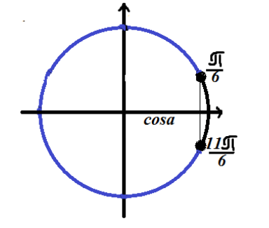
Since the inequality has a “less than” sign, the solution lies on the arc of a circle located to the left (relative to the solution of the equation).
Answer: $\left(\frac(\pi )(6)+2\pi n,\frac(11\pi )(6)+2\pi n\right)$.
Example 3
$tgx\le \frac(\sqrt(3))(3)$
Let's find the solution to the trigonometric inequality $tgx=\frac(\sqrt(3))(3)$
\ \
Here we also need a domain of definition. As we remember, the tangent function $x\ne \frac(\pi )(2)+\pi n,n\in Z$
Let us mark the solution on the trigonometric circle
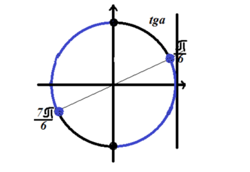
Figure 3. Solution of the inequality $tgx\le \frac(\sqrt(3))(3)$.
Since the inequality has a “less than or equal” sign, the solution lies on the circular arcs marked in blue in Figure 3.
Answer:$\ \left(-\frac(\pi )(2)+2\pi n\right.,\left.\frac(\pi )(6)+2\pi n\right]\cup \left (\frac(\pi )(2)+2\pi n,\right.\left.\frac(7\pi )(6)+2\pi n\right]$
Example 4
Let's find the solution to the trigonometric inequality $ctgx=\sqrt(3)$
\ \
Here we also need a domain of definition. As we remember, the tangent function $x\ne \pi n,n\in Z$
Let us mark the solution on the trigonometric circle
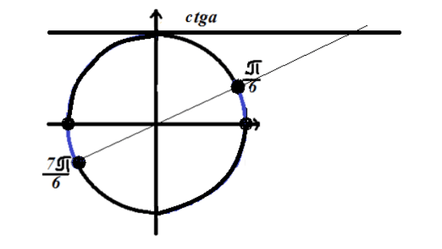
Figure 4. Solution of the inequality $ctgx\le \sqrt(3)$.
Since the inequality has a “greater than” sign, the solution lies on the circular arcs marked in blue in Figure 4.
Answer:$\ \left(2\pi n,\frac(\pi )(6)+2\pi n\right)\cup \left(\pi +2\pi n,\frac(7\pi )( 6)+2\pi n\right)$