Principal component method or component analysis(principal component analysis, PCA) is one of the most important methods in the arsenal of a zoologist or ecologist. Unfortunately, in cases where it is quite appropriate to use component analysis, cluster analysis is often used.

A typical task for which component analysis is useful is this: there is a certain set of objects, each of which is characterized by a certain (sufficiently large) number of characteristics. The researcher is interested in the patterns reflected in the diversity of these objects. In the case when there is reason to assume that objects are distributed among hierarchically subordinate groups, cluster analysis can be used - the method classifications(distribution by groups). If there is no reason to expect that the variety of objects reflects some kind of hierarchy, it is logical to use ordination(orderly arrangement). If each object is characterized sufficiently a large number characteristics (at least so many characteristics that cannot be adequately reflected in one graph), it is optimal to start studying the data with an analysis of the principal components. The fact is that this method is at the same time a method for reducing the dimensionality (number of dimensions) of data.

If a group of objects under consideration is characterized by the values ​​of one characteristic, a histogram (for continuous characteristics) or a bar chart (for characterizing the frequencies of a discrete characteristic) can be used to characterize their diversity. If objects are characterized by two characteristics, a two-dimensional scatter plot can be used, if three, a three-dimensional one can be used. What if there are many signs? You can try to reflect on a two-dimensional graph the relative position of objects relative to each other in multidimensional space. Typically, such a reduction in dimensionality is associated with a loss of information. From different possible ways For such a display, you must choose the one at which the loss of information will be minimal.

Let us explain what was actually said simple example: transition from two-dimensional space to one-dimensional one. The minimum number of points that defines a two-dimensional space (plane) is 3. In Fig. 9.1.1 shows the location of three points on the plane. The coordinates of these points are easy to read from the drawing itself. How to choose a straight line that will carry maximum information about the relative positions of points?

Rice. 9.1.1. Three points on a plane defined by two features. On which line will the maximum dispersion of these points be projected?

Consider the projections of points onto line A (shown in blue). The coordinates of the projections of these points onto line A are: 2, 8, 10. The average value is 6 2 / 3. Variance (2-6 2 / 3)+ (8-6 2 / 3)+ (10-6 2 / 3)=34 2 / 3.

Now consider line B (shown green). Point coordinates - 2, 3, 7; the average value is 4, the variance is 14. Thus, a smaller proportion of the variance is reflected on line B than on line A.

What is this share? Since lines A and B are orthogonal (perpendicular), the shares of the total variance projected onto A and B do not intersect. This means that the total dispersion of the location of the points of interest to us can be calculated as the sum of these two terms: 34 2 / 3 +14 = 48 2 / 3. In this case, 71.2% of the total variance is projected onto line A, and 28.8% onto line B.

How can we determine which line will have the maximum share of variance? This straight line will correspond to the regression line for the points of interest, which is designated C (red). 77.2% of the total variance will be reflected on this line, and this is the maximum possible meaning for a given location of points. Such a straight line onto which the maximum share of the total variance is projected is called first principal component.

And on which line should the remaining 22.8% of the total variance be reflected? On a line perpendicular to the first principal component. This straight line will also be the main component, because the maximum possible share of the variance will be reflected in it (naturally, without taking into account that which was reflected in the first main component). So this is - second principal component.

Having calculated these principal components using Statistica (we will describe the dialogue a little later), we get the picture shown in Fig. 9.1.2. The coordinates of points on the principal components are shown in standard deviations.

Rice. 9.1.2. The location of the three points shown in Fig. 9.1.1, on the plane of two principal components. Why are these points located relative to each other differently than in Fig. 9.1.1?

In Fig. 9.1.2 the relative position of the points appears to be changed. In order to correctly interpret such pictures in the future, one should consider the reasons for the differences in the location of the points in Fig. 9.1.1 and 9.1.2 for more details. Point 1 in both cases is located to the right (has a larger coordinate according to the first sign and the first principal component) than point 2. But, for some reason, point 3 at the original location is lower than the other two points (has smallest value feature 2), and higher than two other points on the plane of the principal components (has a larger coordinate along the second component). This is due to the fact that the principal component method optimizes precisely the dispersion of the original data projected onto the axes it selects. If the principal component is correlated with some original axis, the component and the axis can be directed in the same direction (have a positive correlation) or in opposite directions (have negative correlations). Both of these options are equivalent. The principal component method algorithm may or may not “flip” any plane; no conclusions should be drawn from this.

However, the points in Fig. 9.1.2 are not simply “upside down” compared to their relative positions in Fig. 9.1.1; Their relative positions also changed in a certain way. The differences between the points in the second principal component seem to be enhanced. 22.76% of the total variance accounted for by the second component “spread” the points the same distance as 77.24% of the variance accounted for by the first principal component.

In order for the location of points on the plane of the principal components to correspond to their actual location, this plane would have to be distorted. In Fig. 9.1.3. two concentric circles are shown; their radii are related as shares of the variances reflected by the first and second principal components. Picture corresponding to Fig. 9.1.2, distorted so that standard deviation according to the first principal component it corresponded to a larger circle, and according to the second - to a smaller one.

Rice. 9.1.3. We took into account that the first principal component accounts for b O a larger share of the variance than the second. To do this, we distorted the figure. 9.1.2, fitting it to two concentric circles, the radii of which are related as the proportions of variances attributable to the principal components. But the location of the points still does not correspond to the original one shown in Fig. 9.1.1!

Why is the relative position of the points in Fig. 9.1.3 does not correspond to that in Fig. 9.1.1? In the original figure, Fig. 9.1, the points are located in accordance with their coordinates, and not in accordance with the shares of variance attributable to each axis. A distance of 1 unit according to the first sign (along the x-axis) in Fig. 9.1.1 there is a smaller proportion of the dispersion of points along this axis than the distance of 1 unit according to the second characteristic (along the ordinate). And in Fig. 9.1.1, the distances between points are determined precisely by the units in which the characteristics by which they are described are measured.

Let's complicate the task a little. In table Figure 9.1.1 shows the coordinates of 10 points in 10-dimensional space. The first three points and the first two dimensions are the example we just looked at.

Table 9.1.1. Coordinates of points for further analysis

	Coordinates

For educational purposes, we will first consider only part of the data from the table. 9.1.1. In Fig. 9.1.4 we see the position of ten points on the plane of the first two signs. Please note that the first principal component (line C) went a little differently than in the previous case. No wonder: its position is influenced by all the points being considered.

Rice. 9.1.4. We have increased the number of points. The first principal component goes a little differently, because it was influenced by the added points

In Fig. Figure 9.1.5 shows the position of the 10 points we considered on the plane of the first two components. Notice that everything has changed, not just the proportion of variance accounted for by each principal component, but even the position of the first three points!

Rice. 9.1.5. Ordination in the plane of the first principal components of the 10 points described in Table. 9.1.1. Only the values ​​of the first two characteristics were considered, the last 8 columns of the table. 9.1.1 were not used

In general, this is natural: since the main components are located differently, the relative positions of the points have also changed.

Difficulties in comparing the location of points on the principal component plane and on the original plane of their feature values ​​can cause confusion: why use such a difficult-to-interpret method? The answer is simple. In the event that the objects being compared are described by only two characteristics, it is quite possible to use their ordination according to these initial characteristics. All the advantages of the principal component method appear in the case of multidimensional data. In this case, the principal component method turns out to be effective way reducing data dimensionality.

9.2. Moving to initial data with more dimensions

Let's consider a more complex case: let's analyze the data presented in table. 9.1.1 for all ten characteristics. In Fig. Figure 9.2.1 shows how the window of the method we are interested in is called.

Rice. 9.2.1. Running the principal component method

We will be interested only in the selection of features for analysis, although the Statistica dialog allows for much more fine-tuning (Fig. 9.2.2).

Rice. 9.2.2. Selecting Variables for Analysis

After performing the analysis, a window of its results appears with several tabs (Fig. 9.2.3). All main windows are accessible from the first tab.

Rice. 9.2.3. First tab of the principal component analysis results dialog

You can see that the analysis identified 9 main components, and used them to describe 100% of the variance reflected in the 10 initial characteristics. This means that one sign was superfluous, redundant.

Let's start viewing the results with the “Plot case factor voordinates, 2D” button: it will show the location of points on the plane defined by the two principal components. By clicking this button, we will be taken to a dialog where we will need to indicate which components we will use; It is natural to start the analysis with the first and second components. The result is shown in Fig. 9.2.4.

Rice. 9.2.4. Ordination of the objects under consideration on the plane of the first two principal components

The position of the points has changed, and this is natural: new features are involved in the analysis. In Fig. 9.2.4 reflects more than 65% of the total diversity in the position of the points relative to each other, and this is already a non-trivial result. For example, returning to table. 9.1.1, you can verify that points 4 and 7, as well as 8 and 10, are indeed quite close to each other. However, the differences between them may concern other main components not shown in the figure: they, after all, also account for a third of the remaining variability.

By the way, when analyzing the placement of points on the plane of principal components, it may be necessary to analyze the distances between them. The easiest way to obtain a matrix of distances between points is to use a module for cluster analysis.

How are the identified main components related to the original characteristics? This can be found out by clicking the button (Fig. 9.2.3) Plot var. factor coordinates, 2D. The result is shown in Fig. 9.2.5.

Rice. 9.2.5. Projections of the original features onto the plane of the first two principal components

We look at the plane of the two principal components “from above”. The initial features, which are in no way related to the main components, will be perpendicular (or almost perpendicular) to them and will be reflected in short segments ending near the origin of coordinates. Thus, trait No. 6 is least associated with the first two principal components (although it demonstrates a certain positive correlation with the first component). The segments corresponding to those features that are fully reflected on the plane of the principal components will end on a circle of unit radius enclosing the center of the picture.

For example, you can see that the first principal component was most strongly influenced by features 10 (positively correlated), as well as 7 and 8 (negatively correlated). To consider the structure of such correlations in more detail, you can click the Factor coordinates of variables button and get the table shown in Fig. 9.2.6.

Rice. 9.2.6. Correlations between the initial characteristics and the identified principal components (Factors)

The Eigenvalues ​​button displays values ​​called eigenvalues ​​of the main components. At the top of the window shown in Fig. 9.2.3, the following values ​​are displayed for the first few components; The Scree plot button shows them in an easy-to-read form (Fig. 9.2.7).

Rice. 9.2.7. Eigenvalues ​​of the identified principal components and the share of the total variance reflected by them

First you need to understand what exactly the eigenvalue shows. This is a measure of the variance reflected in the principal component, measured in the amount of variance accounted for by each feature in the initial data. If the eigenvalue of the first principal component is 3.4, this means that it accounts for more variance than the three features in the initial set. Eigenvalues ​​are linearly related to the share of variance attributable to the principal component; the only thing is that the sum of eigenvalues ​​is equal to the number of original features, and the sum of the shares of variance is equal to 100%.

What does it mean that information about variability for 10 characteristics was reflected in 9 principal components? That one of the initial features was redundant did not add any new information. And so it was; in Fig. 9.2.8 shows how the set of points reflected in the table was generated. 9.1.1.

Principal component method(PCA - Principal component analysis) is one of the main ways to reduce the dimension of data with minimal loss of information. Invented in 1901 by Karl Pearson, it is widely used in many fields. For example, for data compression, “computer vision”, visible image recognition, etc. The calculation of the principal components comes down to the calculation of eigenvectors and eigenvalues ​​of the covariance matrix of the original data. The principal component method is often called Karhunen-Löwe ​​transformation(Karhunen-Loeve transform) or Hotelling transformation(Hoteling transform). Mathematicians Kosambi (1943), Pugachev (1953) and Obukhova (1954) also worked on this issue.

The task of principal component analysis aims to approximate (bring closer) data by linear manifolds of lower dimension; find subspaces of lower dimension, in the orthogonal projection on which the spread of data (that is, the standard deviation from the mean value) is maximum; find subspaces of lower dimension, in the orthogonal projection on which the root-mean-square distance between points is maximum. In this case, they operate with finite sets of data. They are equivalent and do not use any hypothesis about the statistical generation of the data.

In addition, the task of principal component analysis may be to construct for a given multidimensional random variable such an orthogonal transformation of coordinates that, as a result, the correlations between individual coordinates will become zero. This version operates random variables.

Fig.3

The above figure shows points P i on the plane, p i is the distance from P i to straight line AB. We are looking for a straight line AB that minimizes the sum

The principal component method began with the problem of the best approximation (approximation) of a finite set of points by straight lines and planes. For example, given a finite set of vectors. For each k = 0,1,...,n? 1 among all k-dimensional linear manifolds in find such that the sum of squared deviations x i from L k is minimal:

Where? Euclidean distance from a point to a linear manifold.

Any k-dimensional linear manifold in can be defined as a set of linear combinations, where the parameters in i run along the real line, huh? orthonormal set of vectors

where is the Euclidean norm? Euclidean dot product, or in coordinate form:

Solution of the approximation problem for k = 0,1,...,n? 1 is given by a set of nested linear manifolds

These linear manifolds are defined by an orthonormal set of vectors (principal component vectors) and a vector a 0 . Vector a 0 is sought as a solution to the minimization problem for L 0:

The result is a sample average:

French mathematician Maurice Fréchet Fréchet Maurice René (09/02/1878 - 06/04/1973) - an outstanding French mathematician. He worked in the field of topology and functional analysis, probability theory. Author modern concepts on metric space, compactness and completeness. Auto. in 1948, he noticed that the variational definition of the mean, as the point that minimizes the sum of squared distances to data points, is very convenient for constructing statistics in an arbitrary metric space, and he built a generalization of classical statistics for general spaces, called the generalized least squares method.

Vectors of principal components can be found as solutions to similar optimization problems:

1) centralize the data (subtract the average):

2) find the first principal component as a solution to the problem;

3) Subtract the projection onto the first principal component from the data:

4) find the second principal component as a solution to the problem

If the solution is not unique, then choose one of them.

2k-1) Subtract the projection onto the (k ? 1)th principal component (recall that the projections onto the previous (k ? 2) principal components have already been subtracted):

2k) find the kth principal component as a solution to the problem:

If the solution is not unique, then choose one of them.

Rice. 4

The first principal component maximizes the sample variance of the data projection.

For example, let us be given a centered set of data vectors where the arithmetic mean x i is zero. Task? find an orthogonal transformation to a new coordinate system for which the following conditions would be true:

1. The sample variance of the data along the first coordinate (principal component) is maximum;

2. The sample dispersion of the data along the second coordinate (second principal component) is maximum under the condition of orthogonality to the first coordinate;

3. The sample dispersion of the data along the values ​​of the k-th coordinate is maximum under the condition of orthogonality to the first k? 1 coordinates;

The sample variance of the data along the direction specified by the normalized vector a k is

(since the data is centered, the sample variance here is the same as the mean square of the deviation from zero).

Solving the best fit problem gives the same set of principal components as finding the orthogonal projections with the greatest scattering, for a very simple reason:

and the first term does not depend on a k.

The data transformation matrix to the principal components is constructed from the vectors “A” of the principal components:

Here a i are orthonormal column vectors of the principal components, arranged in descending order of eigenvalues, the superscript T means transpose. Matrix A is orthogonal: AA T = 1.

After the transformation, most of the data variation will be concentrated in the first coordinates, which makes it possible to discard the remaining ones and consider a reduced-dimensional space.

The oldest method for selecting principal components is Kaiser rule, Kaiser Johann Henrich Gustav (03/16/1853, Brezno, Prussia - 10/14/1940, Germany) - an outstanding German mathematician, physicist, researcher in the field of spectral analysis. Auto. according to which those main components for which are significant

that is, l i exceeds the mean value l (the average sample variance of the data vector coordinates). The Kaiser Rule works well in simple cases, when there are several principal components with l i much greater than the average value, and the remaining eigenvalues ​​are less than it. In more complex cases, it may produce too many significant principal components. If the data are normalized to unit sample variance along the axes, then Kaiser's rule takes on a particularly simple form: only those principal components for which l i > 1 are significant.

One of the most popular heuristic approaches to estimating the number of required principal components is broken cane rule, when the set is normalized to a unit sum eigenvalues(, i = 1,...n) is compared with the distribution of lengths of fragments of a cane of unit length broken at n ? 1st randomly selected point (break points are selected independently and equally distributed along the length of the cane). If L i (i = 1,...n) are the lengths of the resulting cane pieces, numbered in descending order of length: , then the mathematical expectation of L i:

Let's look at an example that involves estimating the number of principal components using the broken cane rule in dimension 5.

Rice. 5.

According to the k-th broken cane rule eigenvector(in descending order of eigenvalues ​​l i) is stored in the list of principal components if

The figure above shows an example for the 5-dimensional case:

l 1 =(1+1/2+1/3+1/4+1/5)/5; l 2 =(1/2+1/3+1/4+1/5)/5; l 3 =(1/3+1/4+1/5)/5;

l 4 =(1/4+1/5)/5; l 5 =(1/5)/5.

For example, selected

0.5; =0.3; =0.1; =0.06; =0.04.

According to the broken cane rule, in this example you should leave 2 main components:

One thing to keep in mind is that the broken cane rule tends to underestimate the number of significant principal components.

After projecting onto the first k principal components c, it is convenient to normalize to unit (sample) variance along the axes. The dispersion along the ith principal component is equal to), so for normalization it is necessary to divide the corresponding coordinate by. This transformation is not orthogonal and does not preserve the dot product. The covariance matrix of the data projection after normalization becomes unit, the projections to any two orthogonal directions become independent quantities, and any orthonormal basis becomes the basis of the principal components (recall that normalization changes the orthogonality relationship of the vectors). The mapping from the source data space to the first k principal components, together with normalization, is given by the matrix

It is this transformation that is most often called the Karhunen-Loeve transformation, that is, the principal component method itself. Here a i are column vectors, and the superscript T means transpose.

In statistics, when using the principal component method, several special terms are used.

Data Matrix, where each row is a vector of preprocessed data (centered and correctly normalized), the number of rows is m (the number of data vectors), the number of columns is n (the dimension of the data space);

Load matrix(Loadings), where each column is a principal component vector, the number of rows is n (the dimension of the data space), the number of columns is k (the number of principal component vectors selected for projection);

Account Matrix(Scores)

where each line is the projection of the data vector onto k principal components; number of rows - m (number of data vectors), number of columns - k (number of principal component vectors selected for projection);

Z-score matrix(Z-scores)

where each row is a projection of the data vector onto k principal components, normalized to unit sample variance; number of rows - m (number of data vectors), number of columns - k (number of principal component vectors selected for projection);

Error Matrix (leftovers) (Errors or residuals)

Basic formula:

Thus, the Principal Component Method is one of the main methods of mathematical statistics. Its main purpose is to distinguish between the need to study data sets with a minimum of their use.

The starting point for analysis is the data matrix

dimensions
, the i-th row of which characterizes the i-th observation (object) for all k indicators
. The source data is normalized, for which the average values ​​of the indicators are calculated
, as well as standard deviation values
. Then the matrix of normalized values

with elements

The matrix of pair correlation coefficients is calculated:

Unit elements are located on the main diagonal of the matrix
.

The component analysis model is constructed by representing the original normalized data as a linear combination of principal components:

Where - “weight”, i.e. factor loading th main component on -th variable;

-meaning th main component for -observation (object), where
.

In matrix form, the model has the form

Here
- matrix of principal components of dimension
,

- matrix of factor loadings of the same dimension.

Matrix
describes observations in space main components. In this case, the matrix elements
are normalized, and the principal components are not correlated with each other. It follows that
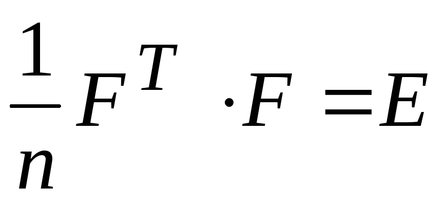, Where – unit matrix of dimension
.

Element matrices characterizes the closeness of the linear relationship between the original variable and the main component , therefore, takes the values
.

Correlation matrix can be expressed through a matrix of factor loadings .

Units are located along the main diagonal of the correlation matrix and, by analogy with the covariance matrix, they represent the variances of the used -features, but unlike the latter, due to normalization, these variances are equal to 1. The total variance of the entire system -features in the sample volume
equal to the sum of these units, i.e. equal to the trace of the correlation matrix
.

The correlation matrix can be transformed into a diagonal matrix, that is, a matrix whose all values, except the diagonal ones, are equal to zero:

,

Where
- a diagonal matrix on the main diagonal of which there are eigenvalues correlation matrix, - a matrix whose columns are eigenvectors of the correlation matrix . Since the matrix R is positive definite, i.e. its leading minors are positive, then all eigenvalues
for any
.

Eigenvalues are found as the roots of the characteristic equation

Eigenvector , corresponding to the eigenvalue correlation matrix , is defined as a nonzero solution to the equation

Normalized eigenvector equals

The vanishing of non-diagonal terms means that the features become independent of each other (
at
).

Total variance of the entire system variables in the sample population remains the same. However, its values ​​are redistributed. The procedure for finding the values ​​of these variances is finding the eigenvalues correlation matrix for each of -signs. The sum of these eigenvalues
is equal to the trace of the correlation matrix, i.e.
, that is, the number of variables. These eigenvalues ​​are the variance values ​​of the features
in conditions if the signs were independent of each other.

In the principal component method, a correlation matrix is ​​first calculated from the original data. Then it is orthogonally transformed and through this the factor loadings are found for all variables and
factors (matrix of factor loadings), eigenvalues and determine the weights of the factors.

The factor loading matrix A can be defined as
, A th column of matrix A - how
.

Weight of factors
or
reflects the share of the total variance contributed by this factor.

Factor loadings vary from –1 to +1 and are analogous to correlation coefficients. In the factor loading matrix, it is necessary to identify significant and insignificant loadings using the Student’s t test
.

Sum of squared loads -th factor in all -features is equal to the eigenvalue of a given factor
. Then
-contribution of the i-th variable in % in the formation of the j-th factor.

The sum of the squares of all factor loadings for a row is equal to one, the total variance of one variable, and of all factors for all variables is equal to the total variance (i.e., the trace or order of the correlation matrix, or the sum of its eigenvalues)
.

In general, the factor structure of the i-th attribute is presented in the form
, which includes only significant loads. Using the matrix of factor loadings, you can calculate the values ​​of all factors for each observation of the original sample population using the formula:

,

Where – value of the j-th factor for the t-th observation, -standardized value of the i-th feature of the t-th observation of the original sample; –factor load, – eigenvalue corresponding to factor j. These calculated values are widely used to graphically represent the results of factor analysis.

Using the matrix of factor loadings, the correlation matrix can be reconstructed:
.

The portion of the variance of a variable explained by the principal components is called the communality

,

Where - variable number, and - number of the main component. The correlation coefficients restored only from the principal components will be less than the original ones in absolute value, and on the diagonal they will not be 1, but the values ​​of the generalities.

Specific contribution - main component is determined by the formula

.

The total contribution of the accounted
the main components are determined from the expression

.

Typically used for analysis
the first principal components, the contribution of which to the total variance exceeds 60-70%.

The factor loading matrix A is used to interpret the principal components, typically considering those values ​​greater than 0.5.

The values ​​of the principal components are specified by the matrix

Main components

5.1 Methods multiple regression and canonical correlation involve dividing the existing set of features into two parts. However, such a division may not always be objectively well-founded, and therefore there is a need for approaches to analyzing the relationships between indicators that would involve considering the vector of characteristics as a single whole. Of course, when implementing such approaches, a certain heterogeneity may be detected in this battery of features when several groups of variables are objectively identified. For characteristics from one such group, cross-correlations will be much higher compared to combinations of indicators from different groups. However, this grouping will be based on the results of an objective data analysis, and not on the a priori arbitrary considerations of the researcher.

5.2 When studying correlations within some single set of m features

X"= X 1 X 2 X 3 ... X m

you can use the same method that was used in multiple regression analysis and the method of canonical correlations - obtaining new variables, the variation of which fully reflects the existence of multivariate correlations.

The purpose of considering intragroup connections of a single set of characteristics is to determine and visually represent the objectively existing main directions of the relative variation of these variables. Therefore, for these purposes, you can introduce some new variables Y i , found as linear combinations of the original set of features X

Y 1 = b 1"X= b 11 X 1 + b 12 X 2 + b 13 X 3 + ... + b 1m X m

Y2= b 2"X= b 21 X 1 + b 22 X 2 + b 23 X 3 + ... + b 2m X m

Y 3 = b 3"X= b 31 X 1 + b 32 X 2 + b 33 X 3 + ... + b 3m X m (5.1)

... ... ... ... ... ... ...

Y m = b m "X= b m1 X 1 + b m2 X 2 + b m3 X 3 + ... + b m m X m

and having a number of desirable properties. For definiteness, let the number of new features be equal to the number of original features (m).

One of these desirable optimal properties may be the mutual uncorrelation of new variables, that is, the diagonal form of their covariance matrix

S y1 2 0 0 ... 0

0 s y2 2 0 ... 0

S y= 0 0 s y3 2 ... 0 , (5.2)

... ... ... ... ...

0 0 0 … s ym 2

where s yi 2 is the variance of the i-th new feature Y i. The uncorrelatedness of new variables, in addition to its obvious convenience, has an important property - each new feature Y i will take into account only its independent part of the information about the variability and correlation of the original indicators X.

The second necessary property of new characteristics is the orderly accounting of variations in the original indicators. Thus, let the first new variable Y 1 take into account the maximum share of the total variation of traits X. This, as we will see later, is equivalent to the requirement that Y 1 have the maximum possible variance s y1 2. Taking into account equality (1.17), this condition can be written in the form

s y1 2 = b 1 "Sb 1= max , (5.3)

Where S- covariance matrix of initial characteristics X, b 1- a vector including coefficients b 11, b 12, b 13, ..., b 1m with the help of which, from the values ​​of X 1, X 2, X 3, ..., X m, the value of Y 1 can be obtained.

Let the second new variable Y 2 describe the maximum part of that component of the total variation that remains after taking into account its largest share in the variability of the first new feature Y 1 . To achieve this, the condition must be met

s y2 2 = b 2 "Sb 2= max , (5.4)

at zero connection Y 1 with Y 2, (i.e. r y1y2 = 0) and at s y1 2 > s y2 2.

Similarly, the third new feature Y 3 should describe the third most important part of the variation of the original features, for which its variance should also be maximum

s y3 2 = b 3 "Sb 3= max , (5.5)

under the conditions that Y 3 is uncorrelated with the first two new features Y 1 and Y 2 (i.e. r y1y3 = 0, r y2y3 = 0) and s y1 2 > s y2 > s y3 2 .

Thus, the variances of all new variables are characterized by ordering in magnitude

s y1 2 > s y2 2 > s y3 2 > ... > s y m 2 . (5.6)

5.3 Vectors from formula (5.1) b 1 , b 2 , b 3 , ..., b m , with the help of which the transition to new variables Y i should be carried out, can be written in the form of a matrix

B = b 1 b 2 b 3 ... b m. (5.7)

Transition from a set of initial features X to a set of new variables Y can be represented as a matrix formula

Y = B" X , (5.8)

and obtaining a covariance matrix of new features and achieving condition (5.2) of uncorrelatedness of new variables in accordance with formula (1.19) can be represented as

B"SB= S y , (5.9)

where is the covariance matrix of the new variables S y due to their uncorrelated nature, it has a diagonal shape. From matrix theory (section A.25 Appendix A) it is known that, having obtained for some symmetric matrix A eigenvectors u i and numbers l i and invert

calling matrices from them U And L, in accordance with formula (A.31) we can obtain the result

U"AU= L ,

Where L- diagonal matrix including eigenvalues ​​of a symmetric matrix A. It is easy to see that the last equality completely coincides with formula (5.9). Therefore, we can draw the following conclusion. Desirable properties of new variables Y can be provided if the vectors b 1 , b 2 , b 3 , ..., b m , with the help of which the transition to these variables should be carried out, will be the eigenvectors of the covariance matrix of the original features S. Then the variances of the new features s yi 2 will turn out to be eigenvalues

s y1 2 = l 1, s y2 2 = l 2, s y3 2 = l 3, ..., s ym 2 = l m (5.10)

New variables, the transition to which according to formulas (5.1) and (5.8) is carried out using the eigenvectors of the covariance matrix of the original features, are called principal components. Due to the fact that the number of eigenvectors of the covariance matrix in general case is equal to m - the number of initial features for this matrix, the number of principal components is also equal to m.

In accordance with matrix theory, to find the eigenvalues ​​and vectors of the covariance matrix, one should solve the equation

(S-l i I)b i = 0 . (5.11)

This equation has a solution if the condition that the determinant is equal to zero is satisfied

½ S-l i I½ = 0. (5.12)

This condition essentially also turns out to be an equation whose roots are all the eigenvalues ​​l 1 , l 2 , l 3 , ..., l m of the covariance matrix simultaneously coinciding with the variances of the principal components. After obtaining these numbers, for each i-th of them, using equation (5.11), you can obtain the corresponding eigenvector b i. In practice, special iteration procedures are used to calculate eigenvalues ​​and vectors (Appendix B).

All eigenvectors can be written as a matrix B, which will be an orthonormal matrix, so (section A.24 Appendix A) is fulfilled for it

B"B = BB" = I . (5.13)

The latter means that for any pair of eigenvectors b i "b j= 0, and for any such vector the equality b i "b i = 1.

5.4 Let us illustrate the derivation of principal components for the simplest case of two initial features X 1 and X 2 . The covariance matrix for this set is

where s 1 and s 2 are the standard deviations of characteristics X 1 and X 2, and r is the correlation coefficient between them. Then condition (5.12) can be written in the form

S 1 2 - l i rs 1 s 2

rs 1 s 2 s 2 2 - l i

Figure 5.1.Geometric meaning of the main components

Expanding the determinant, we can obtain the equation

l 2 - l(s 1 2 + s 2 2) + s 1 2 s 2 2 (1 - r 2) = 0,

solving which, you can get two roots l 1 and l 2. Equation (5.11) can also be written as

s 1 2 - l i r s 1 s 2 b i1 = 0

r s 1 s 2 s 2 2 - l i b i2 0

Substituting l 1 into this equation, we obtain a linear system

(s 1 2 - l 1) b 11 + rs 1 s 2 b 12 = 0

rs 1 s 2 b 11 + (s 2 2 - l 1)b 12 = 0,

the solution of which is the elements of the first eigenvector b 11 and b 12. After a similar substitution of the second root l 2, we find the elements of the second eigenvector b 21 and b 22.

5.5 Let's find out geometric meaning main components. This can be done clearly only for the simplest case of two features X 1 and X 2. Let them be characterized by a bivariate normal distribution with a positive correlation coefficient. If all individual observations are plotted on a plane, formed by axes signs, then the corresponding points will be located inside a certain correlation ellipse (Fig. 5.1). New features Y 1 and Y 2 can also be depicted on the same plane in the form of new axes. According to the meaning of the method, for the first principal component Y 1, which takes into account the maximum possible total dispersion of the characteristics X 1 and X 2, the maximum of its dispersion should be achieved. This means that for Y 1 one should find the

which axis so that the width of the distribution of its values ​​is greatest. Obviously, this will be achieved if this axis coincides in direction with the largest axis of the correlation ellipse. Indeed, if we project all the points corresponding to individual observations onto this coordinate, we will obtain a normal distribution with the maximum possible range and the greatest dispersion. This will be the distribution of individual values ​​of the first principal component Y 1 .

The axis corresponding to the second principal component Y 2 must be drawn perpendicular to the first axis, as this follows from the condition that the principal components are uncorrelated. Indeed, in this case we will obtain a new coordinate system with the Y 1 and Y 2 axes coinciding in direction with the axes of the correlation ellipse. It can be seen that the correlation ellipse, when examined in the new coordinate system, demonstrates the uncorrelatedness of the individual values ​​of Y 1 and Y 2, while for the values ​​of the original characteristics X 1 and X 2 a correlation was observed.

The transition from the axes associated with the original features X 1 and X 2 to a new coordinate system oriented to the main components Y 1 and Y 2 is equivalent to rotating the old axes by a certain angle j. Its value can be found using the formula

Tg 2j = . (5.14)

The transition from the values ​​of features X 1 and X 2 to the main components can be carried out in accordance with the results of analytical geometry in the form

Y 1 = X 1 cos j + X 2 sin j

Y 2 = - X 1 sin j + X 2 cos j.

The same result can be written in matrix form

Y 1 = cos j sin j X 1 and Y 2 = -sin j cos j X 1,

which exactly corresponds to the transformation Y 1 = b 1"X and Y 2 = b 2"X. In other words,

= B" . (5.15)

Thus, the eigenvector matrix can also be interpreted as including trigonometric functions of the angle of rotation that must be made to move from the coordinate system associated with the original features to new axes based on the principal components.

If we have m initial features X 1, X 2, X 3, ..., X m, then the observations that make up the sample under consideration will be located inside some m-dimensional correlation ellipsoid. Then the axis of the first principal component will coincide in direction with the largest axis of this ellipsoid, the axis of the second principal component with the second axis of this ellipsoid, etc. The transition from the original coordinate system associated with the feature axes X 1, X 2, X 3, ..., X m to the new axes of the principal components will be equivalent to several rotations of the old axes at angles j 1, j 2, j 3, .. ., and the transition matrix B from the set X to the system of main components Y, consisting of its own eyelids-

tori of the covariance matrix, includes trigonometric functions of the angles of the new coordinate axes with the old axes of the original features.

5.6 In accordance with the properties of eigenvalues ​​and vectors, the traces of the covariance matrices of the original features and principal components are equal. In other words

tr S= tr S y = tr L (5.16)

s 11 + s 22 + ... + s mm = l 1 + l 2 + ... + l m,

those. the sum of the eigenvalues ​​of the covariance matrix is ​​equal to the sum of the variances of all original features. Therefore, we can talk about a certain total value of the dispersion of the original characteristics equal to tr S, and the system of eigenvalues ​​taken into account.

The fact that the first principal component has a maximum variance equal to l 1 automatically means that it also describes the maximum share of the total variation of the original characteristics tr S. Similarly, the second principal component has the second largest variance l 2, which corresponds to the second largest taken into account share of the total variation of the original characteristics, etc.

For each principal component, it is possible to determine the proportion of the total variability of the original characteristics that it describes

5.7 Obviously, the idea of ​​​​the total variation of a set of initial characteristics X 1, X 2, X 3, ..., X m, measured by the value tr S, makes sense only if all these characteristics are measured in the same units. Otherwise, you will have to add the variances, different signs, some of which will be expressed in squared millimeters, others in squared kilograms, others in squared radians or degrees, etc. This difficulty can be easily avoided if we move from the named values ​​of features X ij to their normalized values ​​z ij = (X ij - M i)./ S i where M i and S i are the arithmetic mean and standard deviation of the i-th feature. Normalized z features have zero means, unit variances, and are not associated with any units of measurement. Covariance matrix of initial features S will turn into a correlation matrix R.

Everything that has been said about the principal components found for the covariance matrix remains true for the matrix R. Here it is exactly the same, based on the eigenvectors of the correlation matrix b 1 , b 2 , b 3 , ..., b m, go from the initial features z i to the main components y 1, y 2, y 3, ..., y m

y 1 = b 1"z

y 2 = b 2"z

y 3 = b 3"z

y m = b m "z .

This transformation can also be written in compact form

y = B"z ,

Figure 5.2. Geometric meaning of the principal components for two normalized features z 1 and z 2

Where y- vector of values ​​of the main components, B- matrix including eigenvectors, z- vector of initial normalized features. Equality turns out to be fair

B"RB= ... ... … , (5.18)

where l 1, l 2, l 3, ..., l m are the eigenvalues ​​of the correlation matrix.

The results obtained by analyzing the correlation matrix differ from similar results for the covariance matrix. First, it is now possible to consider traits measured in different units. Secondly, the eigenvectors and numbers found for the matrices R And S, are also different. Thirdly, the main components determined from the correlation matrix and based on the normalized values ​​of the features z turn out to be centered - i.e. having zero average values.

Unfortunately, having determined the eigenvectors and numbers for the correlation matrix, it is impossible to move from them to similar vectors and numbers of the covariance matrix. In practice, principal components based on a correlation matrix are usually used as they are more universal.

5.8 Let us consider the geometric meaning of the principal components determined from the correlation matrix. The case of two signs z 1 and z 2 is clear here. The coordinate system associated with these normalized features has a zero point located in the center of the graph (Fig. 5.2). The central point of the correlation ellipse,

including all individual observations, will coincide with the center of the coordinate system. Obviously, the axis of the first principal component, which has the maximum variation, will coincide with the largest axis of the correlation ellipse, and the coordinate of the second principal component will be oriented along the second axis of this ellipse.

The transition from the coordinate system associated with the original features z 1 and z 2 to the new axes of the principal components is equivalent to rotating the first axes by a certain angle j. The variances of the normalized features are equal to 1 and using formula (5.14) we can find the value of the rotation angle j equal to 45 o. Then the matrix of eigenvectors, which can be determined through the trigonometric functions of this angle using formula (5.15), will be equal to

Cos j sin j 1 1 1

B" = = .

Sin j cos j (2) 1/2 -1 1

The eigenvalues ​​for the two-dimensional case are also easy to find. Condition (5.12) turns out to be of the form

which corresponds to the equation

l 2 - 2l + 1 - r 2 = 0,

which has two roots

l 1 = 1 + r (5.19)

Thus, the main components of the correlation matrix for two normalized features can be found using very simple formulas

Y 1 = (z 1 + z 2) (5.20)

Y 2 = (z 1 - z 2)

Their arithmetic means are equal to zero, and their standard deviations have the values

s y1 = (l 1) 1/2 = (1 + r) 1/2

s y2 = (l 2) 1/2 = (1 - r) 1/2

5.9 In accordance with the properties of eigenvalues ​​and vectors, the traces of the correlation matrix of the original features and the matrix of eigenvalues ​​are equal. The total variation of m normalized features is equal to m. In other words

tr R= m = tr L (5.21)

l 1 + l 2 + l 3 + ... + l m = m.

Then the share of the total variation of the original characteristics described by the i-th principal component is equal to

You can also introduce the concept of P cn - the share of the total variation of the original characteristics described by the first n principal components,

n l 1 + l 2 + ... + l n

P cn = S P i = . (5.23)

The fact that for eigenvalues ​​an order of the form l 1 > l 2 > > l 3 > ... > l m is observed means that similar relationships will be characteristic of the fractions described by the main components of variation

P 1 > P 2 > P 3 > ... > P m . (5.24)

Property (5.24) entails a specific form of dependence of the accumulated fraction P сn on n (Fig. 5.3). In this case, the first three principal components describe the bulk of the variability of traits. This means that often the first few principal components can jointly account for up to 80 - 90% of the total variation in traits, while each subsequent principal component will increase this proportion very slightly. Then, for further consideration and interpretation, only these first few principal components can be used with confidence that they describe the most important patterns of intragroup variability and correlation

Figure 5.3. Dependence of the share of total variation of traits P cn described by the first n principal components on the value n. Number of features m = 9

Figure 5.4. Towards determining the design of the criterion for screening out the principal components

signs. Thanks to this, the number of informative new variables that need to be worked with can be reduced by 2-3 times. Thus, the main components have one more important and useful property- they significantly simplify the description of variations in initial characteristics and make it more compact. Such a reduction in the number of variables is always desirable, but it is associated with some distortions in the relative positions of points corresponding to individual observations in the space of the first few principal components compared to the m-dimensional space of the original features. These distortions arise from trying to squeeze the feature space into the space of the first principal components. However, in mathematical statistics it is proven that of all the methods that can significantly reduce the number of variables, the transition to principal components leads to the least distortion of the structure of observations associated with this reduction.

5.10 An important issue in the analysis of principal components is the problem of determining their quantity for further consideration. It is obvious that an increase in the number of principal components increases the accumulated share of the taken into account variability P cn and brings it closer to 1. At the same time, the compactness of the resulting description decreases. The choice of the number of main components that simultaneously ensures both completeness and compactness of the description can be based on different criteria used in practice. Let's list the most common ones.

The first criterion is based on the consideration that the number of principal components taken into account should provide sufficient informative completeness of the description. In other words, the principal components under consideration should describe most of the total variability of the original characteristics: up to 75 - 90%. The choice of a specific level of the accumulated share P cn remains subjective and depends both on the opinion of the researcher and on the problem being solved.

Another similar criterion (Kaiser's criterion) allows one to include into consideration principal components with eigenvalues ​​greater than 1. It is based on the consideration that 1 is the variance of one normalized initial feature. This is

Well, the inclusion in further consideration of all principal components with eigenvalues ​​greater than 1 means that we consider only those new variables that have variances of at least one original feature. The Kaiser criterion is very common and its use is included in many statistical data processing software packages when it is necessary to set the minimum value of the eigenvalue taken into account, and the default value is often equal to 1.

Cattell's screening criterion is somewhat better theoretically justified. Its application is based on consideration of a graph on which the values ​​of all eigenvalues ​​are plotted in descending order (Fig. 5.4). Cattell's criterion is based on the effect that a plotted sequence of values ​​of the resulting eigenvalues ​​usually produces a concave line. The first few eigenvalues ​​exhibit a non-linear decrease in their level. However, starting from a certain eigenvalue, the decrease in this level becomes approximately linear and rather flat. The inclusion of the main components in the consideration ends with the one whose eigenvalue begins the rectilinear, flat section of the graph. Thus, in Figure 5.4, in accordance with Cattell’s criterion, only the first three principal components should be included in consideration, because the third eigenvalue is located at the very beginning of the rectilinear flat section of the graph.

The Cattell criterion is based on the following. If we consider data on m characteristics, artificially obtained from a table of normally distributed random numbers, then for them the correlations between the characteristics will be completely random and will be close to 0. If the main components are found here, it will be possible to detect a gradual decrease in the value of their eigenvalues, which has a rectilinear character. In other words, a linear decrease in eigenvalues ​​may indicate the absence of signs of non-random connections in the corresponding information about the correlation.

5.11 When interpreting principal components, eigenvectors are most often used, presented in the form of so-called loads - correlation coefficients of the original features with the principal components. Eigenvectors b i, satisfying equality (5.18), are obtained in normalized form, so that b i "b i= 1. This means that the sum of the squares of the elements of each eigenvector is 1. Eigenvectors whose elements are loads can be easily found using the formula

a i= (l i) 1/2 b i . (5.25)

In other words, by multiplying the normalized form of the eigenvector by the square root of its eigenvalue, one can obtain a set of loadings of the original features onto the corresponding principal component. For load vectors, the following equality is true: a i "a i= l i, meaning that the sum of the squares of the loads on i-th main component is equal to the i-th eigenvalue. Computer programs usually output eigenvectors in the form of loads. If it is necessary to obtain these vectors in normalized form b i this can be done using a simple formula b i = a i/ (l i) 1/2.

5.12 The mathematical properties of eigenvalues ​​and vectors are such that, according to Sect. A.25 Appendix A is the original correlation matrix. R can be represented in the form R = BLB", which can also be written as

R= l 1 b 1 b 1 "+ l 2 b 2 b 2 "+ l 3 b 3 b 3 "+ ... + l m b m b m " . (5.26)

It should be noted that any of the terms l i b i b i ", corresponding to the i-th principal component, is square matrix

L i b i1 2 l i b i1 b i2 l i b i1 b i3 … l i b i1 b im

l i b i b i "= l i b i1 b i2 l i b i2 2 l i b i2 b i3 ... l i b i2 b im . (5.27)

... ... ... ... ...

l i b i1 b im l i b i2 b im l i b i3 b im ... l i b im 2

Here b ij is the element of the i-th eigenvector of the j-th original feature. Any diagonal term of such a matrix l i b ij 2 is a certain fraction of the variation of the j-th attribute described by the i-th principal component. Then the variance of any j-th attribute can be represented as

1 = l 1 b 1j 2 + l 2 b 2j 2 + l 3 b 3j 2 + ... + l m b mj 2 , (5.28)

meaning its expansion into contributions depending on all the main components.

Similarly, any off-diagonal term l i b ij b ik of matrix (5.27) is some part of the correlation coefficient r jk of the j-th and k-th features taken into account by the i-th principal component. Then we can write the expansion of this coefficient as a sum

r jk = l 1 b 1j b 1k + l 2 b 2j b 2k + ... + l m b mj b mk , (5.29)

contributions of all m principal components to it.

Thus, from formulas (5.28) and (5.29) one can clearly see that each principal component describes a certain part of the variance of each original feature and the correlation coefficient of each combination.

Taking into account that the elements of the normalized form of the eigenvectors b ij are related to the loads a ij by simple relation (5.25), expansion (5.26) can also be written in terms of the eigenvectors of the loads R = AA", which can also be represented as

R = a 1 a 1" + a 2 a 2" + a 3 a 3" + ... + a m a m" , (5.30)

those. as the sum of the contributions of each of the m main components. Each of these contributions a i a i " can be written as a matrix

A i1 2 a i1 a i2 a i1 a i3 ... a i1 a im

a i1 a i2 a i2 2 a i2 a i3 ... a i2 a im

a i a i "= a i1 a i3 a i2 a i3 a i3 2 ... a i3 a im , (5.31)

... ... ... ... ...

a i1 a im a i2 a im a i3 a im ... a im 2

on the diagonals of which a ij 2 are placed - contributions to the variance of the j-th original feature, and off-diagonal elements a ij a ik - there are similar contributions to the correlation coefficient r jk of the j-th and k-th features.

Principal component method

Principal component method(English) Principal component analysis, PCA ) is one of the main ways to reduce the dimensionality of data, losing the least amount of information. Invented by K. Pearson Karl Pearson ) in. It is used in many areas, such as pattern recognition, computer vision, data compression, etc. The calculation of principal components comes down to the calculation of eigenvectors and eigenvalues ​​of the covariance matrix of the original data. Sometimes the principal component method is called Karhunen-Loeve transformation(English) Karhunen-Loeve) or the Hotelling transformation (eng. Hotelling transform). Other ways to reduce the dimensionality of data are the method of independent components, multidimensional scaling, as well as numerous nonlinear generalizations: the method of principal curves and manifolds, the method of elastic maps, the search for the best projection (eng. Projection Pursuit), neural network “bottleneck” methods, etc.

Formal statement of the problem

The principal component analysis problem has at least four basic versions:

• approximate data by linear manifolds of lower dimension;
• find subspaces of lower dimension, in the orthogonal projection on which the spread of data (that is, the standard deviation from the mean value) is maximum;
• find subspaces of lower dimension, in the orthogonal projection onto which the root-mean-square distance between points is maximum;
• for a given multidimensional random variable, construct an orthogonal transformation of coordinates such that, as a result, the correlations between individual coordinates become zero.

The first three versions operate with finite data sets. They are equivalent and do not use any hypothesis about the statistical generation of the data. The fourth version operates with random variables. Finite sets appear here as samples from a given distribution, and the solution to the first three problems appears as an approximation to the “true” Karhunen-Loeve transformation. This raises an additional and not entirely trivial question about the accuracy of this approximation.

Approximation of data by linear manifolds

Illustration for the famous work of K. Pearson (1901): given points on a plane, - the distance from to the straight line. We are looking for a direct line that minimizes the sum

The principal component method began with the problem of the best approximation of a finite set of points by lines and planes (K. Pearson, 1901). A finite set of vectors is given. For each of all -dimensional linear manifolds in, find such that the sum of squared deviations from is minimal:

,

where is the Euclidean distance from a point to a linear manifold. Any -dimensional linear manifold can be defined as a set of linear combinations, where the parameters run along the real line, and is an orthonormal set of vectors

,

where the Euclidean norm is the Euclidean scalar product, or in coordinate form:

.

The solution to the approximation problem for is given by a set of nested linear manifolds , . These linear manifolds are defined by an orthonormal set of vectors (principal component vectors) and a vector. The vector is sought as a solution to the minimization problem for:

.

Vectors of principal components can be found as solutions to similar optimization problems:

1) centralize the data (subtract the average): . Now ; 2) find the first principal component as a solution to the problem; . If the solution is not unique, then choose one of them. 3) Subtract from the data the projection onto the first principal component: ; 4) find the second principal component as a solution to the problem. If the solution is not unique, then choose one of them. … 2k-1) Subtract the projection onto the th principal component (recall that the projections onto the previous principal components have already been subtracted): ; 2k) find the kth principal component as a solution to the problem: . If the solution is not unique, then choose one of them. ...

At each preparatory step, we subtract the projection onto the previous principal component. The found vectors are orthonormalized simply as a result of solving the described optimization problem, however, in order to prevent calculation errors from disturbing the mutual orthogonality of the vectors of the main components, they can be included in the conditions of the optimization problem.

Non-uniqueness in the definition, in addition to the trivial arbitrariness in the choice of sign (and they solve the same problem), can be more significant and arise, for example, from the conditions of data symmetry. The last principal component is a unit vector orthogonal to all previous ones.

Finding orthogonal projections with the greatest scattering

The first principal component maximizes the sample variance of the data projection

Let us be given a centered set of data vectors (the arithmetic mean is zero). The task is to find an orthogonal transformation to a new coordinate system for which the following conditions would be true:

The theory of singular value decomposition was created by J. J. Sylvester. James Joseph Sylvester ) in the city and is stated in all detailed guides on matrix theory.

A simple iterative singular value decomposition algorithm

The main procedure is to search for the best approximation of an arbitrary matrix by a matrix of the form (where - -dimensional vector, and - -dimensional vector) using the least squares method:

The solution to this problem is given by successive iterations using explicit formulas. For a fixed vector, the values ​​that provide a minimum to the form are uniquely and explicitly determined from the equalities:

Similarly, with a fixed vector, the values ​​are determined:

As an initial approximation of the vector, we take a random vector of unit length, calculate the vector, then for this vector we calculate the vector, etc. Each step reduces the value. The stopping criterion is the smallness of the relative decrease in the value of the minimized functional per iteration step () or the smallness of the value itself.

As a result, we obtained the best approximation for the matrix using a matrix of the form (here the superscript denotes the approximation number). Next, we subtract the resulting matrix from the matrix, and for the resulting deviation matrix we again look for the best approximation of the same type, etc., until, for example, the norm becomes sufficiently small. As a result, we obtained an iterative procedure for decomposing a matrix in the form of a sum of matrices of rank 1, that is, . We assume and normalize the vectors: As a result, an approximation of singular numbers and singular vectors (right - and left -) is obtained.

The advantages of this algorithm include its exceptional simplicity and the ability to transfer it almost without changes to data with spaces, as well as weighted data.

There are various modifications to the basic algorithm that improve accuracy and robustness. For example, the vectors of the main components for different should be orthogonal “by construction”, however, for large number iterations (high dimension, many components), small deviations from orthogonality accumulate and a special correction may be required at each step to ensure its orthogonality to the previously found principal components.

Singular decomposition of tensors and the tensor method of principal components

Often the data vector has the additional structure of a rectangular table (for example, a flat image) or even a multidimensional table - that is, a tensor: , . In this case, it is also effective to use singular value decomposition. The definition, basic formulas and algorithms are transferred practically without changes: instead of a data matrix, we have an index value , where the first index is the number of the data point (tensor).

The main procedure is to search for the best approximation of a tensor by a tensor of the form (where is a -dimensional vector ( is the number of data points), is a dimension vector at ) using the least squares method:

The solution to this problem is given by successive iterations using explicit formulas. If all factor vectors are given except one, then this remaining one is determined explicitly from sufficient conditions for the minimum.

As an initial approximation of vectors (), we take random vectors of unit length, calculate the vector, then for this vector and these vectors we calculate the vector, etc. (cyclically iterating through the indices) Each step reduces the value of . The algorithm obviously converges. The stopping criterion is the smallness of the relative decrease in the value of the minimized functional per cycle or the smallness of the value itself. Next, we subtract the resulting approximation from the tensor and again look for the best approximation of the same type for the remainder, etc., until, for example, the norm of the next remainder becomes sufficiently small.

This multicomponent singular value decomposition (tensor principal component method) is successfully used in processing images, video signals, and, more broadly, any data that has a tabular or tensor structure.

Transformation matrix to principal components

The data transformation matrix to principal components consists of vectors of principal components, arranged in descending order of eigenvalues:

(means transpose),

That is, the matrix is ​​orthogonal.

Most of the data variation will be concentrated in the first coordinates, which allows you to move to a lower-dimensional space.

Residual variance

Let the data be centered, . When replacing data vectors with their projection onto the first principal components, the average squared error is introduced per one data vector:

where are the eigenvalues ​​of the empirical covariance matrix , arranged in descending order, taking into account multiplicity.

This quantity is called residual variance. Magnitude

called explained variance. Their sum is equal to the sample variance. The corresponding squared relative error is the ratio of the residual variance to the sample variance (i.e. proportion of unexplained variance):

The relative error evaluates the applicability of the principal component method with projection onto the first components.

Comment: In most computational algorithms, eigenvalues ​​with corresponding eigenvectors - principal components - are calculated in order from largest to smallest. To calculate it, it is enough to calculate the first eigenvalues ​​and the trace of the empirical covariance matrix (the sum of the diagonal elements, that is, the variances along the axes). Then

Selection of principal components according to Kaiser's rule

The target approach to estimating the number of principal components based on the required proportion of explained variance is always formally applicable, but it implicitly assumes that there is no separation into “signal” and “noise”, and any predetermined accuracy makes sense. Therefore, another heuristic is often more productive, based on the hypothesis of the presence of a “signal” (relatively small dimension, relatively large amplitude) and “noise” (large dimension, relatively small amplitude). From this point of view, the principal component method works like a filter: the signal is contained mainly in the projection onto the first principal components, and the proportion of noise in the remaining components is much higher.

Question: how to estimate the number of required principal components if the signal-to-noise ratio is unknown in advance?

The simplest and oldest method for selecting principal components gives Kaiser rule(English) Kaiser's rule): those main components are significant for which

that is, it exceeds the mean (average sample variance of the data vector coordinates). Kaiser's rule works well in simple cases where there are several principal components with , much larger than the average, and the remaining eigenvalues ​​are less than it. In more complex cases, it may produce too many significant principal components. If the data are normalized to unit sample variance along the axes, then Kaiser's rule takes on a particularly simple form: only those principal components for which

Estimating the number of principal components using the broken cane rule

Example: estimating the number of principal components using the broken cane rule in dimension 5.

One of the most popular heuristic approaches to estimating the number of required principal components is broken cane rule(English) Broken stick model) . The set of eigenvalues ​​normalized to the unit sum (, ) is compared with the distribution of fragment lengths of a cane of unit length broken at the th randomly selected point (the break points are chosen independently and are equally distributed along the length of the cane). Let () be the lengths of the resulting pieces of cane, numbered in descending order of length: . It is not difficult to find the mathematical expectation:

By the broken cane rule, the th eigenvector (in descending order of eigenvalues) is stored in the list of principal components if

In Fig. An example is given for the 5-dimensional case:

=(1+1/2+1/3+1/4+1/5)/5; =(1/2+1/3+1/4+1/5)/5; =(1/3+1/4+1/5)/5; =(1/4+1/5)/5; =(1/5)/5.

For example, selected

=0.5; =0.3; =0.1; =0.06; =0.04.

According to the broken cane rule, in this example you should leave 2 main components:

According to user ratings, the broken cane rule tends to underestimate the number of significant principal components.

Normalization

Normalization after reduction to principal components

After projection onto the first principal components with it is convenient to normalize to unit (sample) variance along the axes. The dispersion along the th main component is equal to ), so for normalization it is necessary to divide the corresponding coordinate by . This transformation is not orthogonal and does not preserve the dot product. The covariance matrix of the data projection after normalization becomes unit, the projections to any two orthogonal directions become independent quantities, and any orthonormal basis becomes the basis of the principal components (recall that normalization changes the orthogonality relationship of the vectors). The mapping from the source data space to the first principal components, together with normalization, is specified by the matrix

.

It is this transformation that is most often called the Karhunen-Loeve transformation. Here are column vectors, and the superscript means transpose.

Normalization before calculating principal components

Warning: one should not confuse the normalization carried out after transformation to the principal components with normalization and “non-dimensionalization” when data preprocessing, carried out before calculating the principal components. Preliminary normalization is needed to make a reasonable choice of the metric in which the best approximation of the data will be calculated, or the directions of the greatest scatter will be sought (which is equivalent). For example, if the data are three-dimensional vectors of "meters, liters and kilograms", then using standard Euclidean distance, a difference of 1 meter in the first coordinate will contribute the same as a difference of 1 liter in the second, or 1 kg in the third . Typically, the systems of units in which the original data are presented do not accurately reflect our ideas about the natural scales along the axes, and “dimensionless” is carried out: each coordinate is divided into a certain scale determined by the data, the purposes of their processing and the processes of measurement and data collection.

There are three significantly different standard approaches to such normalization: unit variance along the axes (the scales along the axes are equal to the mean square deviations - after this transformation, the covariance matrix coincides with the matrix of correlation coefficients), on equal measurement accuracy(the scale along the axis is proportional to the accuracy of measurement of a given value) and on equal demands in the problem (the scale along the axis is determined by the required accuracy of the forecast of a given value or its permissible distortion - the level of tolerance). The choice of preprocessing is influenced by the meaningful formulation of the problem, as well as the conditions of data collection (for example, if the data collection is fundamentally incomplete and data will still be received, then it is irrational to choose normalization strictly to unit variance, even if this corresponds to the meaning of the problem, since this involves renormalization of all data after receiving a new portion; it is more reasonable to choose some scale that roughly estimates standard deviation, and do not change it further).

Pre-normalization to unit variance along the axes is destroyed by rotation of the coordinate system if the axes are not principal components, and normalization during data preprocessing does not replace normalization after normalization to principal components.

Mechanical analogy and principal component analysis for weighted data

If we assign a unit mass to each data vector, then the empirical covariance matrix coincides with the inertia tensor of this point mass system (divided by the total mass), and the problem of principal components coincides with the problem of reducing the inertia tensor to the principal axes. You can use additional freedom in choosing mass values ​​to take into account the importance of data points or the reliability of their values ​​(important data or data from more reliable sources are assigned larger masses). If the data vector is given mass, then instead of the empirical covariance matrix we get

All further operations for reduction to the principal components are carried out in the same way as in the main version of the method: we look for an orthonormal eigenbasis, order it in descending order of eigenvalues, estimate the weighted average error of data approximation by the first components (based on the sums of eigenvalues), normalize, etc. .

A more general method of weighing gives maximizing the weighted sum of pairwise distances between projections. For every two data points, a weight is entered; And . Instead of the empirical covariance matrix, we use

When the symmetric matrix is ​​positive definite, since the quadratic form is positive:

Next, we look for an orthonormal eigenbasis, arrange it in descending order of eigenvalues, estimate the weighted average error of data approximation by the first components, etc. - exactly the same as in the main algorithm.

This method is used if there are classes: for different classes the weight is chosen to be greater than for points of the same class. As a result, in the projection onto the weighted principal components, the different classes are “moved apart” by a greater distance.

Other uses - reducing the impact of large deviations(outlayers, English) Outlier ), which can distort the picture due to the use of the root mean square distance: if you choose , the influence of large deviations will be reduced. Thus, the described modification of the principal component method is more robust than the classical one.

Special terminology

In statistics, when using the principal component method, several special terms are used.

Data Matrix; each line is a vector preprocessed data ( centered and right standardized), number of rows - (number of data vectors), number of columns - (dimension of data space);

Load matrix(Loadings) ; each column is a vector of principal components, the number of rows is (the dimension of the data space), the number of columns is (the number of vectors of principal components selected for projection);

Account Matrix(Scores); each line is a projection of the data vector onto the principal components; number of rows - (number of data vectors), number of columns - (number of principal component vectors selected for projection);

Z-score matrix(Z-scores); each line is a projection of the data vector onto the principal components, normalized to the unit sample variance; number of rows - (number of data vectors), number of columns - (number of principal component vectors selected for projection);

Error Matrix(or leftovers) (Errors or residuals) .

Basic formula:

Limits of applicability and limitations of the effectiveness of the method

The principal component method is always applicable. The common claim that it applies only to normally distributed data (or for distributions close to normal) is incorrect: in the original formulation of K. Pearson the problem is set: approximations finite set of data and there is not even a hypothesis about their statistical generation, not to mention their distribution.

However, the method is not always effective in reducing dimensionality given the accuracy constraints. Straight lines and planes do not always provide a good approximation. For example, data may follow a curve with good accuracy, but this curve may be difficult to locate in data space. In this case, the principal component method for acceptable accuracy will require several components (instead of one), or will not reduce the dimensionality at all with acceptable accuracy. To deal with such "curved" principal components, the principal manifold method and various versions of the nonlinear principal component method were invented. Complex topology data can cause more trouble. Various methods have also been invented to approximate them, such as self-organizing Kohonen maps, neural gas or topological grammars. If the data is statistically generated with a distribution that is very different from normal, then to approximate the distribution it is useful to move from principal components to independent components, which are no longer orthogonal in the original scalar product. Finally, for an isotropic distribution (even a normal one), instead of a scattering ellipsoid we get a ball, and it is impossible to reduce the dimension by approximation methods.

Examples of using

Data visualization

Data visualization is a visual representation of experimental data or the results of theoretical research.

The first choice in visualizing a data set is to orthogonally project onto a plane the first two principal components (or 3-dimensional space of the first three main component). The design plane is essentially a flat two-dimensional “screen” positioned in such a way as to provide a “picture” of the data with the least distortion. Such a projection will be optimal (among all orthogonal projections on different two-dimensional screens) in three respects:

1. The sum of the squares of the distances from the data points to the projections onto the plane of the first principal components is minimal, that is, the screen is located as close as possible to the point cloud.
2. The sum of distortions of the squared distances between all pairs of points from the data cloud after projecting the points onto the plane is minimal.
3. The sum of distortions of the squared distances between all data points and their “center of gravity” is minimal.

Data visualization is one of the most widely used applications of principal component analysis and its nonlinear generalizations.

Image and video compression

To reduce spatial redundancy of pixels when encoding images and videos, linear transformations of pixel blocks are used. Subsequent quantization of the obtained coefficients and lossless coding allows one to obtain significant compression ratios. Using the PCA transform as a linear transform is, for some data types, optimal in terms of the size of the resulting data while maintaining the same distortion. At the moment, this method is not actively used, mainly due to its high computational complexity. Data compression can also be achieved by discarding the last conversion coefficients.

Reduce noise in images

Chemometrics

The principal component method is one of the main methods in chemometrics. Chemometrics ). Allows you to divide the source data matrix X into two parts: “meaningful” and “noise”. According to the most popular definition, “Chemometrics is a chemical discipline that applies mathematical, statistical and other methods based on formal logic to construct or select optimal measurement methods and experimental designs, as well as to extract the most important information in the analysis of experimental data.”

Psychodiagnostics

1. data analysis (describing the results of surveys or other studies presented in the form of numerical data arrays);
2. description of social phenomena (construction of models of phenomena, including mathematical models).

In political science, the principal component method was the main tool of the “Political Atlas of Modernity” project for linear and nonlinear analysis of ratings of 192 countries of the world according to five specially developed integral indices (standard of living, international influence, threats, statehood and democracy). To map the results of this analysis, a special GIS (Geographic Information System) has been developed, combining geographic space with feature space. Political atlas data maps have also been created using two-dimensional main manifolds in the five-dimensional space of countries as a base. The difference between a data map and a geographic map is that geographical map objects that have similar geographic coordinates appear nearby, while on the data map there are objects (countries) with similar characteristics (indices) nearby.